Introduction
The package was designed to make EMODnet vector data layers easily
accessible in R. The package allows users to query information on and
download data from all available EMODnet
Web Feature Service (WFS) endpoints directly into their R working
environment. Data are managed as sf objects which
are currently the state-of-the-art in handling of vector spatial data in
R. The package also allows user to specify the coordinate reference
system of imported data.
Installation
You can install the development version of emodnet.wfs from GitHub with:
pak::pak("EMODnet/emodnet.wfs")Explore the EMODnet WFS services with R
For this tutorial we will make use of the sf and mapview
packages. The simple features sf package is a well known
standard for dealing with geospatial vector data. To visualize
geometries, mapview will create quick interactive maps.
Run this line to install these packages:
install.packages(c("sf", "mapview"))EMODnet is organized into seven thematic lots: Bathymetry, Geology, Seabed Habitats, Chemistry, Biology, Physics, and Human Activities, each focusing on a specific aspect of marine data. With the emodnet.wfs package, we can explore and combine the data served by the EMODnet thematic lots through OGC Web Feature Services or WFS.
Imagine we are interested in seabed substrates. The first step is to
choose what EMODnet thematic lot can provide with these data. For that,
we can check the services available with the emodnet_wfs()
function.
library(emodnet.wfs)
library(mapview)
library(sf)

services <- emodnet_wfs()
class(services)
#> [1] "tbl_df"     "tbl"        "data.frame"
names(services)
#> [1] "emodnet_thematic_lot" "service_name"         "service_url"
services[, c("emodnet_thematic_lot", "service_name")]
#> # A tibble: 17 × 2
#>    emodnet_thematic_lot     service_name
#>    <chr>                    <chr>
#>  1 EMODnet Bathymetry       bathymetry
#>  2 EMODnet Biology          biology
#>  3 EMODnet Biology          biology_occurrence_data
#>  4 EMODnet Chemistry        chemistry_cdi_data_discovery_and_access_service
#>  5 EMODnet Chemistry        chemistry_cdi_distribution_observations_per_category_and_re…
#>  6 EMODnet Chemistry        chemistry_contaminants
#>  7 EMODnet Chemistry        chemistry_marine_litter
#>  8 EMODnet Geology          geology_coastal_behavior
#>  9 EMODnet Geology          geology_events_and_probabilities
#> 10 EMODnet Geology          geology_marine_minerals
#> 11 EMODnet Geology          geology_sea_floor_bedrock
#> 12 EMODnet Geology          geology_seabed_substrate_maps
#> 13 EMODnet Geology          geology_submerged_landscapes
#> 14 EMODnet Human Activities human_activities
#> 15 EMODnet Physics          physics
#> 16 EMODnet Seabed Habitats  seabed_habitats_general_datasets_and_products
#> 17 EMODnet Seabed Habitats  seabed_habitats_individual_habitat_map_and_model_datasets
EMODnet data covers several disciplines organized in 7 thematic lots:
bathymetry, biology, chemistry, geology, human activities, physics,
seabed habitats. Some thematic lots organize their data in more than one
data source or service. The column service_name shows
services available, while service_url has the corresponding
base url to perform a WFS request. The Seabed portal should have the
data we are looking for. A WFS client can be created by passing the
corresponding service_name to the function
emodnet_init_wfs_client(). The layers available to this WFS
client are consulted with emodnet_get_wfs_info().
seabed_wfs_client <- emodnet_init_wfs_client(service = "seabed_habitats_general_datasets_and_products")
#> ✔ WFS client created successfully
#> ℹ Service: "https://ows.emodnet-seabedhabitats.eu/geoserver/emodnet_open/wfs"
#> ℹ Version: "2.0.0"

emodnet_get_wfs_info(wfs = seabed_wfs_client)
#> # A tibble: 72 × 9
#> # Rowwise:
#>    data_source service_name           service_url layer_name title abstract class format
#>    <chr>       <chr>                  <chr>       <chr>      <chr> <chr>    <chr> <chr>
#>  1 emodnet_wfs seabed_habitats_gener… https://ow… art17_hab… 2013… "Gridde… WFSF… sf
#>  2 emodnet_wfs seabed_habitats_gener… https://ow… art17_hab… 2013… "Gridde… WFSF… sf
#>  3 emodnet_wfs seabed_habitats_gener… https://ow… art17_hab… 2013… "Gridde… WFSF… sf
#>  4 emodnet_wfs seabed_habitats_gener… https://ow… art17_hab… 2013… "Gridde… WFSF… sf
#>  5 emodnet_wfs seabed_habitats_gener… https://ow… art17_hab… 2013… "Gridde… WFSF… sf
#>  6 emodnet_wfs seabed_habitats_gener… https://ow… art17_hab… 2013… "Gridde… WFSF… sf
#>  7 emodnet_wfs seabed_habitats_gener… https://ow… art17_hab… 2013… "Gridde… WFSF… sf
#>  8 emodnet_wfs seabed_habitats_gener… https://ow… art17_hab… 2013… "Gridde… WFSF… sf
#>  9 emodnet_wfs seabed_habitats_gener… https://ow… carib_eus… 2023… "Output… WFSF… sf
#> 10 emodnet_wfs seabed_habitats_gener… https://ow… biogenic_… Biog… "This l… WFSF… sf
#> # ℹ 62 more rows
#> # ℹ 1 more variable: layer_namespace <chr>
Each layer is explained in the abstract column. We can
see several layers with the information provided by the EU member states
for the Habitats
Directive 92/43/EEC reporting. We will select the layers about
coastal lagoons, mudflats and sandbanks with their respective
layer_name.
habitats_directive_layer_names <- c("art17_hab_1110", "art17_hab_1140", "art17_hab_1150")

emodnet_get_layer_info(
  wfs = seabed_wfs_client,
  layers = habitats_directive_layer_names
)
#> # A tibble: 3 × 9
#> # Rowwise:
#>   data_source service_name            service_url layer_name title abstract class format
#>   <chr>       <chr>                   <chr>       <chr>      <chr> <chr>    <chr> <chr>
#> 1 emodnet_wfs https://ows.emodnet-se… seabed_hab… art17_hab… 2013… "Gridde… WFSF… sf
#> 2 emodnet_wfs https://ows.emodnet-se… seabed_hab… art17_hab… 2013… "Gridde… WFSF… sf
#> 3 emodnet_wfs https://ows.emodnet-se… seabed_hab… art17_hab… 2013… "Gridde… WFSF… sf
#> # ℹ 1 more variable: layer_namespace <chr>
We are now ready to read the layers into R with
emodnet_get_layers(). emodnet.wfs reads the geometries as
simple features (See sf package) transformed to 4326 by default. Specifying another map
projection is possible by passing a EPGS code or projection string with
emodnet_get_layers(crs = "your projection") where crs is a
coordinate reference system (CRS). The argument
simplify = TRUE stack all the layers in one single tibble.
Default is FALSE and returns a list of sf objects, one per layer.
habitats_directive_layers <- emodnet_get_layers(
  wfs = seabed_wfs_client,
  layers = habitats_directive_layer_names,
  simplify = TRUE,
  outputFormat = "application/json"
)
#> Start tag expected, '<' not found
#> Start tag expected, '<' not found
#> Start tag expected, '<' not found

habitats_directive_layers
#> Simple feature collection with 221 features and 8 fields
#> Geometry type: MULTIPOLYGON
#> Dimension:     XY
#> Bounding box:  xmin: 950000 ymin: 940000 xmax: 6510000 ymax: 4820000
#> Projected CRS: ETRS89-extended / LAEA Europe
#> First 10 features:
#>                   id habitat_code ms region cs_ms   country_code
#> 1  art17_hab_1110.13         1110 DK    ATL   U2+        Denmark
#> 2  art17_hab_1110.22         1110 ES    MAC   U1+          Spain
#> 3  art17_hab_1110.25         1110 ES   MMAC   U1+          Spain
#> 4  art17_hab_1110.59         1110 PT   MMAC    XX       Portugal
#> 5  art17_hab_1110.56         1110 PT   MATL   U1-       Portugal
#> 6  art17_hab_1110.53         1110 PL   MBAL   U1-         Poland
#> 7  art17_hab_1110.17         1110 DK   MBAL   U1-        Denmark
#> 8  art17_hab_1110.31         1110 FR   MATL   U1x         France
#> 9  art17_hab_1110.75         1110 UK   MATL   U1x United Kingdom
#> 10  art17_hab_1110.1         1110 BE    ATL   U1x        Belgium
#>                                                  habitat_code_uri
#> 1  http://dd.eionet.europa.eu/vocabulary/art17_2018/habitats/1110
#> 2  http://dd.eionet.europa.eu/vocabulary/art17_2018/habitats/1110
#> 3  http://dd.eionet.europa.eu/vocabulary/art17_2018/habitats/1110
#> 4  http://dd.eionet.europa.eu/vocabulary/art17_2018/habitats/1110
#> 5  http://dd.eionet.europa.eu/vocabulary/art17_2018/habitats/1110
#> 6  http://dd.eionet.europa.eu/vocabulary/art17_2018/habitats/1110
#> 7  http://dd.eionet.europa.eu/vocabulary/art17_2018/habitats/1110
#> 8  http://dd.eionet.europa.eu/vocabulary/art17_2018/habitats/1110
#> 9  http://dd.eionet.europa.eu/vocabulary/art17_2018/habitats/1110
#> 10 http://dd.eionet.europa.eu/vocabulary/art17_2018/habitats/1110
#>                                               habitat_description
#> 1  Sandbanks which are slightly covered by sea water all the time
#> 2  Sandbanks which are slightly covered by sea water all the time
#> 3  Sandbanks which are slightly covered by sea water all the time
#> 4  Sandbanks which are slightly covered by sea water all the time
#> 5  Sandbanks which are slightly covered by sea water all the time
#> 6  Sandbanks which are slightly covered by sea water all the time
#> 7  Sandbanks which are slightly covered by sea water all the time
#> 8  Sandbanks which are slightly covered by sea water all the time
#> 9  Sandbanks which are slightly covered by sea water all the time
#> 10 Sandbanks which are slightly covered by sea water all the time
#>                          geometry
#> 1  MULTIPOLYGON (((4200000 360...
#> 2  MULTIPOLYGON (((1950000 950...
#> 3  MULTIPOLYGON (((1960000 950...
#> 4  MULTIPOLYGON (((1810000 120...
#> 5  MULTIPOLYGON (((2730000 173...
#> 6  MULTIPOLYGON (((4610000 346...
#> 7  MULTIPOLYGON (((4310000 352...
#> 8  MULTIPOLYGON (((3790000 314...
#> 9  MULTIPOLYGON (((3780000 319...
#> 10 MULTIPOLYGON (((3800000 313...
Note the use of the outputFormat argument in this
example. This specifies the file type to request from the service, which
can influence how the data is loaded into R. By default, the data is
provided in the GML format with a geometry type of
“MULTISURFACE.” However, this geometry type is not widely supported by
many software tools, including the mapview package. To
address this, you can request a different file type, such as GeoJSON,
which delivers the geometry as “MULTIPOLYGON”—a format that is more
universally compatible. This has been raised before in the sf community.
Run the following code to have a quick look at the layers geometries.
mapview(habitats_directive_layers, zcol = "habitat_description", burst = TRUE)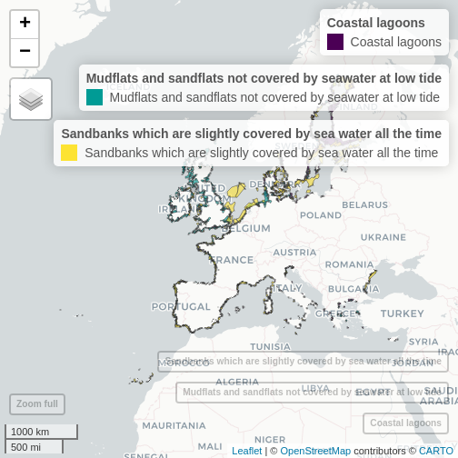
plot of chunk unnamed-chunk-6
EMODnet provides also physics, chemistry, biological or bathymetry data. Explore all the layers available with:
emodnet_get_all_wfs_info()
#> # A tibble: 1,713 × 9
#> # Rowwise:
#>    data_source service_name service_url           layer_name title abstract class format
#>    <chr>       <chr>        <chr>                 <chr>      <chr> <chr>    <chr> <chr>
#>  1 emodnet_wfs bathymetry   https://ows.emodnet-… download_… Bath… "Downlo… WFSF… sf
#>  2 emodnet_wfs bathymetry   https://ows.emodnet-… contours   Dept… "Genera… WFSF… sf
#>  3 emodnet_wfs bathymetry   https://ows.emodnet-… hr_bathym… High… "Layer … WFSF… sf
#>  4 emodnet_wfs bathymetry   https://ows.emodnet-… quality_i… Qual… "Repres… WFSF… sf
#>  5 emodnet_wfs bathymetry   https://ows.emodnet-… sea_names  Sea … "Mainta… WFSF… sf
#>  6 emodnet_wfs bathymetry   https://ows.emodnet-… source_re… Sour… "Covera… WFSF… sf
#>  7 emodnet_wfs bathymetry   https://ows.emodnet-… undersea_… unde… ""       WFSF… sf
#>  8 emodnet_wfs biology      https://geo.vliz.be/… mediseh_c… EMOD… "Coral … WFSF… sf
#>  9 emodnet_wfs biology      https://geo.vliz.be/… mediseh_c… EMOD… "Coral … WFSF… sf
#> 10 emodnet_wfs biology      https://geo.vliz.be/… mediseh_c… EMOD… "Cymodo… WFSF… sf
#> # ℹ 1,703 more rows
#> # ℹ 1 more variable: layer_namespace <chr>
More information
References
Blondel, Emmanuel. (2020, May 27). ows4R: R Interface to OGC Web-Services (Version 0.1-5). Zenodo. https://doi.org/10.5281/zenodo.3860330
Flanders Marine Institute (2019). Maritime Boundaries Geodatabase, version 11. Available online at https://www.marineregions.org/. https://doi.org/10.14284/382.
Hadley Wickham, Romain François, Lionel Henry and Kirill Müller (2020). dplyr: A Grammar of Data Manipulation. R package version 1.0.2.https://CRAN.R-project.org/package=dplyr
Pebesma E (2018). “Simple Features for R: Standardized Support for Spatial Vector Data.” The R Journal, 10(1), 439–446. doi: 10.32614/RJ-2018-009, https://doi.org/10.32614/RJ-2018-009.
R Core Team (2020). R: A language and environment for statistical computing. R Foundation for Statistical Computing, Vienna, Austria. URL https://www.R-project.org/.
Tim Appelhans, Florian Detsch, Christoph Reudenbach and Stefan Woellauer (2020). mapview: Interactive Viewing of Spatial Data in R. R package version 2.9.0. https://CRAN.R-project.org/package=mapview
Code
To cite emodnet.wfs, please use the output from
citation(package = "emodnet.wfs").
citation(package = "emodnet.wfs")
#> To cite package 'emodnet.wfs' in publications use:
#>
#>   Krystalli A, Fernández-Bejarano S, Salmon M (????). _emodnet.wfs: Access
#>   EMODnet Web Feature Service data through R_. doi:10.14284/679
#>   <https://doi.org/10.14284/679>, R package version 2.0.2.9000. Integrated
#>   data products created under the European Marine Observation Data Network
#>   (EMODnet) Biology project (EASME/EMFF/2017/1.3.1.2/02/SI2.789013), funded by
#>   the by the European Union under Regulation (EU) No 508/2014 of the European
#>   Parliament and of the Council of 15 May 2014 on the European Maritime and
#>   Fisheries Fund, <https://github.com/EMODnet/emodnet.wfs>.
#>
#> A BibTeX entry for LaTeX users is
#>
#>   @Manual{,
#>     title = {{emodnet.wfs}: Access EMODnet Web Feature Service data through R},
#>     author = {Anna Krystalli and Salvador Fernández-Bejarano and Maëlle Salmon},
#>     note = {R package version 2.0.2.9000. Integrated data products created under the European Marine Observation Data Network (EMODnet) Biology project (EASME/EMFF/2017/1.3.1.2/02/SI2.789013), funded by the by the European Union under Regulation (EU) No 508/2014 of the European Parliament and of the Council of 15 May 2014 on the European Maritime and Fisheries Fund},
#>     url = {https://github.com/EMODnet/emodnet.wfs},
#>     doi = {10.14284/679},
#>   }