The ICES northsea benthic survey (NSBS) from 1986, including abiotic conditions.
NSBSdensitydata.RdThe NSBS Northsea macrobenthos data (1986).
Samples are within (-3 and 9) dgE and (51.00 60.75) dgN
The data contain:
Macrofauna species density and biomass (
NSBS$density,NSBS$biomass)Abiotic conditions (
NSBS$abiotics), and station positions (NSBS$stations)NSBS$contours: contourlines for mapping.NSBS$fishing: species trait values that can be used to estimate fishing parameters.
NSBS$sar: station-specific fishing intensities.
data(NSBS)Format
==================
**NSBS$density**:
This is the main Northsea NSBS benthos data set, containing species information for 234 stations sampled in 1985-1986.
The data, in long format, are in a data.frame with the following columns:
station, the NSBS station name (details in NSBS$stations).date, the sampling date (year).taxon, the taxon name to be used (usually species), and checked against the WoRMS database (details in datasetTaxonomy).density, the number of individuals per m2.
==================
**NSBS$biomass**:
This data set, contains biomass data for 214 stations sampled in 1985-1986.
Biomass information is on higher taxonomic level. The distinction is made between Crustacea, Polychaeta, Animalia, Mollusca, Echinodermata.
The data, in long format, are in a data.frame with the following columns:
station, the NSBS station name (details in NSBS$stations).date, the sampling date (year).taxon, the taxon name to be used (5 higher taxa).biomass, the biomass, gAFDW/m2.
==================
**NSBS$abiotics**:
the abiotic conditions of sampling stations.
NSBS$abiotics is a data.frame with the following columns:
station, the NSBS station name
depth, water depth, [m]
D50, Median grain size, [micrometer]
mud, mud content of sediment (<63 um), fraction, [-]
sand, sand fraction (64 -2000 um), [-]
gravel, gravel fraction (>2000 um), [-]
salinity, salinity
porosity, volumetric water content, [-]
permeability, sediment permeability, [m2]
POC, particulate organic C in sediment, [percent]
TN, total N in sediment, [percent]
surfaceCarbon, particulate organic C in upper cm, [percent]
surfaceNitrogen, total N in upper cm, [percent]
orbitalVelMean, mean orbital velocity, [m/s]
orbitalVelMax, maximal orbital velocity, [m/s]
tidalVelMean, mean tidal velocity, [m/s]
tidalVelMax, maximal tidal velocity, [m/s]
bedstress, bed shear stress, [Pa]
EUNIScode, EUNIScode, [-]
DRB, swept area ratio for dredge, [m2/m2/year]
OT, swept area ratio for otter trawl, [m2/m2/year]
SN, swept area ratio for seines, [m2/m2/year]
TBB, swept area ratio for beam trawl, [m2/m2/year]
sar, total swept area ratio , DRB +OT +SN +TBB, [m2/m2/year]
subsar, swept area ratio (fisheries) > 2cm, [m2/m2/year]
gpd, gear penetration depth, [cm]
The fishing data (sar, subsar, gpd) were derived from ICES upon request by OSPAR.
They are averaged over (2009-2018). See also NSBS$sar.
==================
**NSBS$fishing**:
species trait values that can be used to estimate fishing parameters.
==================
**NSBS$stations**:
The positions of the different stations, in WGS84 format
station, the NSBS station name
x, degrees longitude
y, degrees latitude
==================
**NSBS$contours**:
The data for mapping the contours. The contourlines (x-, y) were derived from GEBCO high-resolution bathymetry, by creating contourlines.
The data set contains:
station, the NSBS station name
x: longitude, in [dgE]
y: latitude, in [dgN]
z: the corresponding depths, in [m]
==================
**NSBS$sar**:
Fishing data for the NSBS stations, origin: ICES upon request by OSPAR. The NSBS stations nearest to the ICES data were selected.
A data.frame that contains:
station, the NSBS station name
year: the fishing year
gear: metier; TBB, OT: beam, otter trawl; DRB: dredge, SN: seine.
sar: annual swept area ratios (m2/m2/yr) for the surface (0-2cm).
subsar: annual swept area ratios (m2/m2/yr) for the subsurface (>2cm).
gpd: estimated gear penetration depths ([cm]), based on metier
Note
The dataset **Taxonomy**:
contains taxonomic information of the original and adjusted taxon in NSBS$density,
as derived from the World Register of Marine Species (WoRMS), using R-package worrms.
Details
NSBS contains the *macrofauna data* from the 1986 North Sea Benthos Survey, an activity of the Benthos Ecology Working Group of ICES.
Benthic samples were taken in a standardised way, on a regular grid covering the whole of the North Sea, and analysed by scientists from 10 laboratories. Extensive work was done to standardise taxonomy and identifications across the different laboratories.
Sediment was sampled with a Reineck Boxcorer (0,078 m2). Macrofauna sieved on a 1 mm mesh.
=====================================================================
The *fishing data* (in abiotics and sar) were derived from ICES upon request by OSPAR.
They are averaged over (2009-2018).
The metiers are Aggregated into beam trawl (TBB), dredge (DRB), demersal seine (SN), and otter trawl (OT), based on the metier layers: OT_CRU, OT_DMF, OT_MIX, OT_MIX_CRU, OT_MIX_DMF_BEN, OT_MIX_DMF_PEL, OT_MIX_CRU_DMF, OT_SPF, TBB_CRU, TBB_DMF, TBB_MOL, DRB_MOL, SDN_DMF, SSC_DMF
The gear penetration depths used were the mean values over sand and muddy sediments:
in sand: 3.5, 1.1, 1.1, 1.9 cm for DRB, OT, SN, TBB respectively
in mud : 5.4, 2.0, 2.0, 3.2 cm for DRB, OT, SN, TBB respectively
References
The taxonomic information was created using the worrms package:
Chamberlain S, Vanhoorne. B (2023). worrms: World Register of Marine Species (WoRMS) Client_. R package version 0.4.3, <https://CRAN.R-project.org/package=worrms>.
The NSBS data are described in:
Heip, C.H.R.; Basford, D.; Craeymeersch, J.A.; Dewarumez, J.-M.; Dorjes, J.; de Wilde, P.; Duineveld, G.; Eleftheriou, A.; Herman, P.M.J.; Kingston, K.; Niermann, U.; Kunitzer, A.; Rachor, E.; Rumohr, H.; Soetaert, K.; Soltwedel, T. (1992). Trends in biomass, density and diversity of North Sea macrofauna. ICES J. Mar. Sci./J. Cons. int. Explor. Mer 49: 13-22
The fishing data were derived from:
ICES Technical Service, Greater North Sea and Celtic Seas Ecoregions, 29 August 2018 sr.2018.14 Version 2: 22 January 2019 https://doi.org/10.17895/ices.pub.4508 OSPAR request on the production of spatial data layers of fishing intensity/pressure.
See also
map_key for plotting.
Traits_nioz for the trait datasets.
get_density for functions operating on these data.
get_Db_index for extracting bioturbation and bioirrigation indices.
long2wide for functions changing the appearance on these data.
Examples
##-----------------------------------------------------
## Show contents of the data set
##-----------------------------------------------------
metadata(NSBS$abiotics)
#> name description units
#> 1 depth water depth m
#> 2 D50 Median grain size micrometer
#> 3 mud mud fraction (<63 um) -
#> 4 sand sand fraction (64 -2000 um) -
#> 5 gravel gravel fraction (>2000 um) -
#> 6 salinity salinity
#> 7 porosity volumetric water content -
#> 8 permeability permeability m2
#> 9 POC particulate organic C in sediment %
#> 10 TN total N in sediment %
#> 11 surfaceCarbon particulate organic C in upper cm %
#> 12 surfaceNitrogen total N in upper cm %
#> 13 orbitalVelMean mean orbital velocity m/s
#> 14 orbitalVelMax maximal orbital velocity m/s
#> 15 tidalVelMean mean tidal velocity m/s
#> 16 tidalVelMax maximal tidal velocity m/s
#> 17 bedstress bed shear stress Pa
#> 18 EUNIScode EUNIScode -
#> 19 DRB swept area ratio for dredge m2/m2/year
#> 20 OT swept area ratio for otter trawl m2/m2/year
#> 21 SN swept area ratio for seines m2/m2/year
#> 22 TBB swept area ratio for beam trawl m2/m2/year
#> 191 sar swept area ratio (fisheries), DRB +OT +SN +TBB m2/m2/year
#> 201 subsar swept area ratio (fisheries) > 2cm m2/m2/year
#> 211 gpd gear penetration depth cm
metadata(NSBS$density)
#> name description units
#> 1 station station name
#> 2 date sampling date, a string
#> 3 taxon taxon name, checked by worms, and adjusted
#> 4 density species total density individuals/m2
##-----------------------------------------------------
## SPECIES data
##-----------------------------------------------------
head(NSBS$density)
#> station date taxon density
#> 1 ICES002 1986 Clitellata 1.0
#> 2 ICES002 1986 Thecostraca 24.0
#> 3 ICES003 1986 Ophiura albida 1.3
#> 4 ICES003 1986 Thecostraca 278.0
#> 5 ICES003 1986 Abludomelita 1.3
#> 6 ICES003 1986 Glycera 6.3
# The number of species per station (over all years)
Nspecies <- tapply(X = NSBS$density$taxon,
INDEX = NSBS$density$station,
FUN = function(x)length(unique(x)))
summary(Nspecies)
#> Min. 1st Qu. Median Mean 3rd Qu. Max.
#> 1.00 30.25 43.00 43.09 55.75 96.00
# The number of times a species has been found
Nocc <- tapply(X = NSBS$density$station,
INDEX = NSBS$density$taxon,
FUN = length)
head(sort(Nocc, decreasing = TRUE)) #most often encountered taxa
#> Spiophanes bombyx Scoloplos armiger Pholoe Goniada maculata
#> 217 196 188 185
#> Ampharetidae Amphiura filiformis
#> 183 183
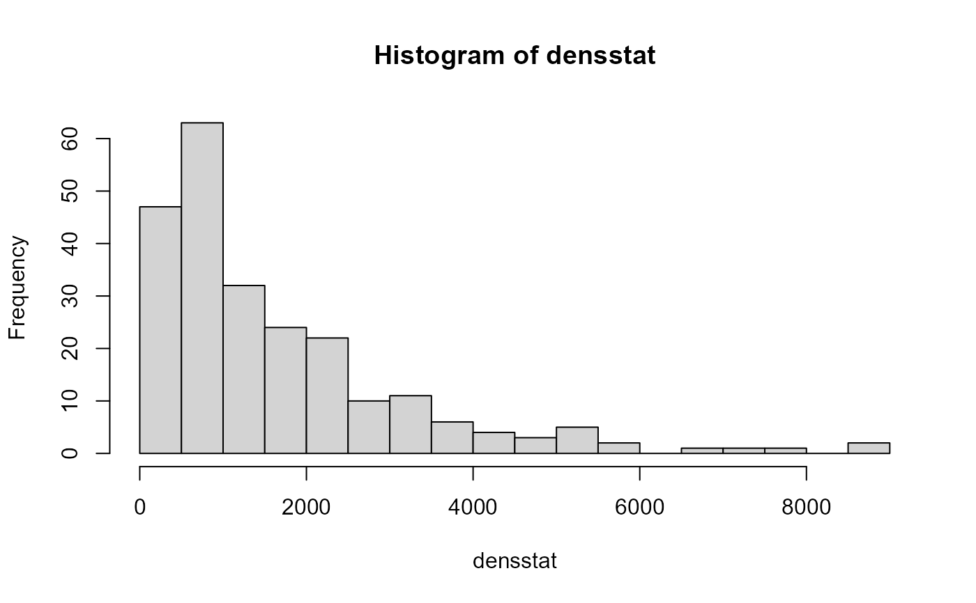
# total density per station
densstat <- tapply(X = NSBS$density$density,
INDEX = list(NSBS$density$station),
FUN = sum)
hist(densstat, n=30)
 ##-----------------------------------------------------
## ABIOTICS
##-----------------------------------------------------
summary(NSBS$abiotics)
#> station depth D50 mud
#> Length :235 Min. : 4.20 Min. :0.03516 Min. :0.0002652
#> N.unique :235 1st Qu.: 34.75 1st Qu.:0.14024 1st Qu.:0.0139084
#> N.blank : 0 Median : 57.50 Median :0.18710 Median :0.0349855
#> Min.nchar: 7 Mean : 63.76 Mean :0.29469 Mean :0.0771892
#> Max.nchar: 7 3rd Qu.: 84.85 3rd Qu.:0.27823 3rd Qu.:0.0872650
#> Max. :195.20 Max. :5.58824 Max. :0.9003331
#> NAs :3 NAs :1 NAs :1
#> sand gravel porosity permeability
#> Min. : 9.86 Min. :0.0000000 Min. :0.3661 Min. :-4.770e-08
#> 1st Qu.:85.57 1st Qu.:0.0005158 1st Qu.:0.3925 1st Qu.: 1.000e-13
#> Median :93.09 Median :0.0055984 Median :0.4110 Median : 2.000e-13
#> Mean :88.38 Mean :0.0389908 Mean :0.4202 Mean : 8.635e-08
#> 3rd Qu.:96.71 3rd Qu.:0.0350953 3rd Qu.:0.4358 3rd Qu.: 1.300e-12
#> Max. :99.97 Max. :0.5836318 Max. :0.7029 Max. : 1.688e-05
#> NAs :1 NAs :1
#> POC TN surfaceCarbon surfaceNitrogen
#> Min. :0.04682 Min. :0.01100 Min. :0.07304 Min. :0.01815
#> 1st Qu.:0.22743 1st Qu.:0.03796 1st Qu.:0.35539 1st Qu.:0.05845
#> Median :0.29917 Median :0.04300 Median :0.46386 Median :0.06793
#> Mean :0.33695 Mean :0.04895 Mean :0.50761 Mean :0.07394
#> 3rd Qu.:0.41622 3rd Qu.:0.05631 3rd Qu.:0.64319 3rd Qu.:0.08698
#> Max. :1.02022 Max. :0.12488 Max. :1.40612 Max. :0.20045
#> NAs :1 NAs :1 NAs :1 NAs :1
#> orbitalVelMean orbitalVelMax tidalVelMean tidalVelMax
#> Min. :0.003484 Min. :0.06843 Min. :0.07054 Min. :0.1619
#> 1st Qu.:0.020203 1st Qu.:0.19295 1st Qu.:0.13072 1st Qu.:0.2938
#> Median :0.037795 Median :0.32866 Median :0.16890 Median :0.3936
#> Mean :0.053431 Mean :0.40298 Mean :0.21072 Mean :0.4741
#> 3rd Qu.:0.063635 3rd Qu.:0.51756 3rd Qu.:0.25985 3rd Qu.:0.5859
#> Max. :0.660648 Max. :2.74205 Max. :0.60274 Max. :1.2783
#> NAs :1 NAs :1 NAs :1 NAs :1
#> bedstress EUNIScode DRB OT
#> Min. :0.00213 Length :235 Min. :0.00000 Min. : 0.00000
#> 1st Qu.:0.07000 N.unique : 7 1st Qu.:0.00000 1st Qu.: 0.03568
#> Median :0.14000 N.blank : 0 Median :0.00000 Median : 0.23662
#> Mean :0.30296 Min.nchar: 4 Mean :0.01122 Mean : 0.90483
#> 3rd Qu.:0.33500 Max.nchar: 4 3rd Qu.:0.00000 3rd Qu.: 0.84740
#> Max. :2.58000 NAs : 1 Max. :0.89844 Max. :15.35263
#> NAs :3
#> SN TBB sar subsar
#> Min. :0.000000 Min. : 0.000000 Min. :8.994e-04 Min. :0.0001127
#> 1st Qu.:0.004945 1st Qu.: 0.000000 1st Qu.:2.701e-01 1st Qu.:0.0354806
#> Median :0.033281 Median : 0.003574 Median :7.277e-01 Median :0.1480871
#> Mean :0.238614 Mean : 0.327851 Mean :1.483e+00 Mean :0.4213943
#> 3rd Qu.:0.146487 3rd Qu.: 0.240855 3rd Qu.:1.731e+00 3rd Qu.:0.5427376
#> Max. :4.550313 Max. :15.298959 Max. :1.548e+01 Max. :8.0287908
#>
#> gpd
#> Min. :1.550
#> 1st Qu.:1.550
#> Median :1.589
#> Mean :1.863
#> 3rd Qu.:2.215
#> Max. :4.382
#>
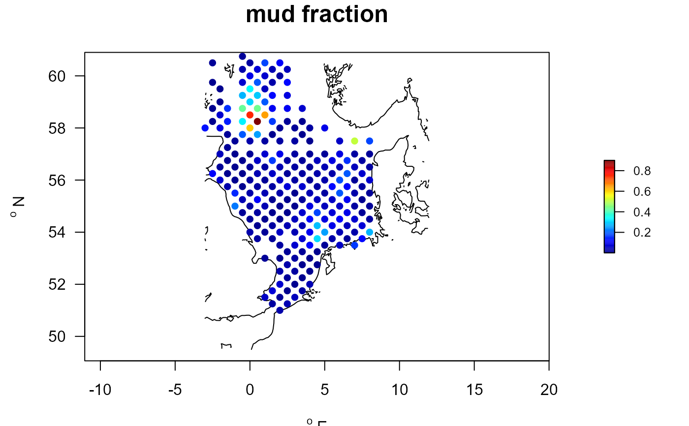
NSBSab <- merge(NSBS$stations, NSBS$abiotics)
with(NSBSab,
map_key(x, y, colvar = mud,
contours = NSBS$contours,
main = "mud fraction",
pch = 16))
##-----------------------------------------------------
## ABIOTICS
##-----------------------------------------------------
summary(NSBS$abiotics)
#> station depth D50 mud
#> Length :235 Min. : 4.20 Min. :0.03516 Min. :0.0002652
#> N.unique :235 1st Qu.: 34.75 1st Qu.:0.14024 1st Qu.:0.0139084
#> N.blank : 0 Median : 57.50 Median :0.18710 Median :0.0349855
#> Min.nchar: 7 Mean : 63.76 Mean :0.29469 Mean :0.0771892
#> Max.nchar: 7 3rd Qu.: 84.85 3rd Qu.:0.27823 3rd Qu.:0.0872650
#> Max. :195.20 Max. :5.58824 Max. :0.9003331
#> NAs :3 NAs :1 NAs :1
#> sand gravel porosity permeability
#> Min. : 9.86 Min. :0.0000000 Min. :0.3661 Min. :-4.770e-08
#> 1st Qu.:85.57 1st Qu.:0.0005158 1st Qu.:0.3925 1st Qu.: 1.000e-13
#> Median :93.09 Median :0.0055984 Median :0.4110 Median : 2.000e-13
#> Mean :88.38 Mean :0.0389908 Mean :0.4202 Mean : 8.635e-08
#> 3rd Qu.:96.71 3rd Qu.:0.0350953 3rd Qu.:0.4358 3rd Qu.: 1.300e-12
#> Max. :99.97 Max. :0.5836318 Max. :0.7029 Max. : 1.688e-05
#> NAs :1 NAs :1
#> POC TN surfaceCarbon surfaceNitrogen
#> Min. :0.04682 Min. :0.01100 Min. :0.07304 Min. :0.01815
#> 1st Qu.:0.22743 1st Qu.:0.03796 1st Qu.:0.35539 1st Qu.:0.05845
#> Median :0.29917 Median :0.04300 Median :0.46386 Median :0.06793
#> Mean :0.33695 Mean :0.04895 Mean :0.50761 Mean :0.07394
#> 3rd Qu.:0.41622 3rd Qu.:0.05631 3rd Qu.:0.64319 3rd Qu.:0.08698
#> Max. :1.02022 Max. :0.12488 Max. :1.40612 Max. :0.20045
#> NAs :1 NAs :1 NAs :1 NAs :1
#> orbitalVelMean orbitalVelMax tidalVelMean tidalVelMax
#> Min. :0.003484 Min. :0.06843 Min. :0.07054 Min. :0.1619
#> 1st Qu.:0.020203 1st Qu.:0.19295 1st Qu.:0.13072 1st Qu.:0.2938
#> Median :0.037795 Median :0.32866 Median :0.16890 Median :0.3936
#> Mean :0.053431 Mean :0.40298 Mean :0.21072 Mean :0.4741
#> 3rd Qu.:0.063635 3rd Qu.:0.51756 3rd Qu.:0.25985 3rd Qu.:0.5859
#> Max. :0.660648 Max. :2.74205 Max. :0.60274 Max. :1.2783
#> NAs :1 NAs :1 NAs :1 NAs :1
#> bedstress EUNIScode DRB OT
#> Min. :0.00213 Length :235 Min. :0.00000 Min. : 0.00000
#> 1st Qu.:0.07000 N.unique : 7 1st Qu.:0.00000 1st Qu.: 0.03568
#> Median :0.14000 N.blank : 0 Median :0.00000 Median : 0.23662
#> Mean :0.30296 Min.nchar: 4 Mean :0.01122 Mean : 0.90483
#> 3rd Qu.:0.33500 Max.nchar: 4 3rd Qu.:0.00000 3rd Qu.: 0.84740
#> Max. :2.58000 NAs : 1 Max. :0.89844 Max. :15.35263
#> NAs :3
#> SN TBB sar subsar
#> Min. :0.000000 Min. : 0.000000 Min. :8.994e-04 Min. :0.0001127
#> 1st Qu.:0.004945 1st Qu.: 0.000000 1st Qu.:2.701e-01 1st Qu.:0.0354806
#> Median :0.033281 Median : 0.003574 Median :7.277e-01 Median :0.1480871
#> Mean :0.238614 Mean : 0.327851 Mean :1.483e+00 Mean :0.4213943
#> 3rd Qu.:0.146487 3rd Qu.: 0.240855 3rd Qu.:1.731e+00 3rd Qu.:0.5427376
#> Max. :4.550313 Max. :15.298959 Max. :1.548e+01 Max. :8.0287908
#>
#> gpd
#> Min. :1.550
#> 1st Qu.:1.550
#> Median :1.589
#> Mean :1.863
#> 3rd Qu.:2.215
#> Max. :4.382
#>
NSBSab <- merge(NSBS$stations, NSBS$abiotics)
with(NSBSab,
map_key(x, y, colvar = mud,
contours = NSBS$contours,
main = "mud fraction",
pch = 16))
 metadata(NSBS$abiotics)
#> name description units
#> 1 depth water depth m
#> 2 D50 Median grain size micrometer
#> 3 mud mud fraction (<63 um) -
#> 4 sand sand fraction (64 -2000 um) -
#> 5 gravel gravel fraction (>2000 um) -
#> 6 salinity salinity
#> 7 porosity volumetric water content -
#> 8 permeability permeability m2
#> 9 POC particulate organic C in sediment %
#> 10 TN total N in sediment %
#> 11 surfaceCarbon particulate organic C in upper cm %
#> 12 surfaceNitrogen total N in upper cm %
#> 13 orbitalVelMean mean orbital velocity m/s
#> 14 orbitalVelMax maximal orbital velocity m/s
#> 15 tidalVelMean mean tidal velocity m/s
#> 16 tidalVelMax maximal tidal velocity m/s
#> 17 bedstress bed shear stress Pa
#> 18 EUNIScode EUNIScode -
#> 19 DRB swept area ratio for dredge m2/m2/year
#> 20 OT swept area ratio for otter trawl m2/m2/year
#> 21 SN swept area ratio for seines m2/m2/year
#> 22 TBB swept area ratio for beam trawl m2/m2/year
#> 191 sar swept area ratio (fisheries), DRB +OT +SN +TBB m2/m2/year
#> 201 subsar swept area ratio (fisheries) > 2cm m2/m2/year
#> 211 gpd gear penetration depth cm
##-----------------------------------------------------
## COMBINATIONS
##-----------------------------------------------------
NSsp_abi <- merge(NSBS$density, NSBS$abiotics)
ECH <- subset(NSsp_abi,
subset = taxon=="Echinocardium cordatum")
with(ECH,
plot(mud, density,
main = "E. cordatum",
xlab = "mud fraction", ylab = "density, ind/m2",
pch = 16))
metadata(NSBS$abiotics)
#> name description units
#> 1 depth water depth m
#> 2 D50 Median grain size micrometer
#> 3 mud mud fraction (<63 um) -
#> 4 sand sand fraction (64 -2000 um) -
#> 5 gravel gravel fraction (>2000 um) -
#> 6 salinity salinity
#> 7 porosity volumetric water content -
#> 8 permeability permeability m2
#> 9 POC particulate organic C in sediment %
#> 10 TN total N in sediment %
#> 11 surfaceCarbon particulate organic C in upper cm %
#> 12 surfaceNitrogen total N in upper cm %
#> 13 orbitalVelMean mean orbital velocity m/s
#> 14 orbitalVelMax maximal orbital velocity m/s
#> 15 tidalVelMean mean tidal velocity m/s
#> 16 tidalVelMax maximal tidal velocity m/s
#> 17 bedstress bed shear stress Pa
#> 18 EUNIScode EUNIScode -
#> 19 DRB swept area ratio for dredge m2/m2/year
#> 20 OT swept area ratio for otter trawl m2/m2/year
#> 21 SN swept area ratio for seines m2/m2/year
#> 22 TBB swept area ratio for beam trawl m2/m2/year
#> 191 sar swept area ratio (fisheries), DRB +OT +SN +TBB m2/m2/year
#> 201 subsar swept area ratio (fisheries) > 2cm m2/m2/year
#> 211 gpd gear penetration depth cm
##-----------------------------------------------------
## COMBINATIONS
##-----------------------------------------------------
NSsp_abi <- merge(NSBS$density, NSBS$abiotics)
ECH <- subset(NSsp_abi,
subset = taxon=="Echinocardium cordatum")
with(ECH,
plot(mud, density,
main = "E. cordatum",
xlab = "mud fraction", ylab = "density, ind/m2",
pch = 16))
 # add station coordinates
ECH <- merge(ECH, NSBS$stations)
##-----------------------------------------------------
## From long format to wide format (stations x species)
##-----------------------------------------------------
NSwide <- with (NSBS$density,
l2w_density(descriptor = station, # long2wide for density
taxon = taxon,
value = density))
PP <- princomp(t(NSwide[,-1]))
if (FALSE) { # \dontrun{
biplot(PP)
} # }
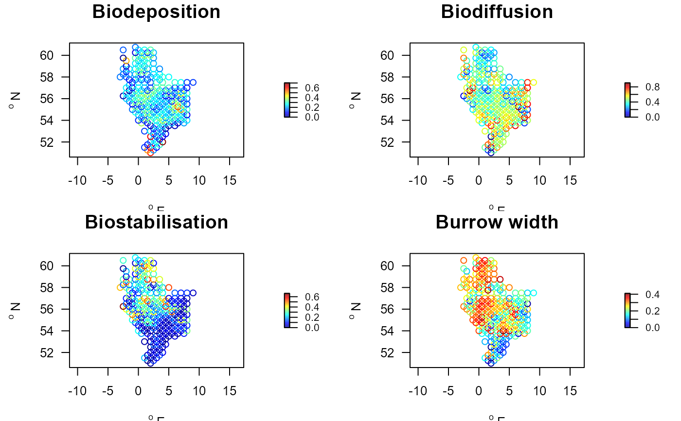
##-----------------------------------------------------
## Community mean weighted score for traits.
##-----------------------------------------------------
# Traits estimated for absences, by including taxonomy
Trait.lab <- metadata(Traits_nioz)
trait.cwm <- get_trait_density(wide = NSwide,
trait = Traits_nioz,
taxonomy = NSBS$taxonomy,
trait_class = Trait.lab$trait,
trait_score = Trait.lab$score,
scalewithvalue = TRUE)
head(trait.cwm, n = c(3, 4))
#> descriptor Age.at.maturity Annual.fecundity Biodeposition
#> 1 ICES002 0.2466667 0.4373333 0.6000000
#> 2 ICES003 0.2898844 0.4404432 0.5120424
#> 3 ICES004 0.1556037 0.3284367 0.1960335
Stations.traits <- merge(NSBS$stations, trait.cwm,
by.x = "station", by.y = "descriptor")
par(mfrow=c(2,2))
with(Stations.traits,
map_key(x, y, colvar = Biodeposition,
main = "Biodeposition"))
#> Warning: no non-missing arguments to min; returning Inf
#> Warning: no non-missing arguments to max; returning -Inf
with(Stations.traits,
map_key(x, y, colvar = Biodiffusion,
main = "Biodiffusion"))
#> Warning: no non-missing arguments to min; returning Inf
#> Warning: no non-missing arguments to max; returning -Inf
with(Stations.traits,
map_key(x, y, colvar = Biostabilisation,
main = "Biostabilisation"))
#> Warning: no non-missing arguments to min; returning Inf
#> Warning: no non-missing arguments to max; returning -Inf
with(Stations.traits,
map_key(x, y, colvar = Burrow.width,
main = "Burrow width"))
#> Warning: no non-missing arguments to min; returning Inf
#> Warning: no non-missing arguments to max; returning -Inf
# add station coordinates
ECH <- merge(ECH, NSBS$stations)
##-----------------------------------------------------
## From long format to wide format (stations x species)
##-----------------------------------------------------
NSwide <- with (NSBS$density,
l2w_density(descriptor = station, # long2wide for density
taxon = taxon,
value = density))
PP <- princomp(t(NSwide[,-1]))
if (FALSE) { # \dontrun{
biplot(PP)
} # }
##-----------------------------------------------------
## Community mean weighted score for traits.
##-----------------------------------------------------
# Traits estimated for absences, by including taxonomy
Trait.lab <- metadata(Traits_nioz)
trait.cwm <- get_trait_density(wide = NSwide,
trait = Traits_nioz,
taxonomy = NSBS$taxonomy,
trait_class = Trait.lab$trait,
trait_score = Trait.lab$score,
scalewithvalue = TRUE)
head(trait.cwm, n = c(3, 4))
#> descriptor Age.at.maturity Annual.fecundity Biodeposition
#> 1 ICES002 0.2466667 0.4373333 0.6000000
#> 2 ICES003 0.2898844 0.4404432 0.5120424
#> 3 ICES004 0.1556037 0.3284367 0.1960335
Stations.traits <- merge(NSBS$stations, trait.cwm,
by.x = "station", by.y = "descriptor")
par(mfrow=c(2,2))
with(Stations.traits,
map_key(x, y, colvar = Biodeposition,
main = "Biodeposition"))
#> Warning: no non-missing arguments to min; returning Inf
#> Warning: no non-missing arguments to max; returning -Inf
with(Stations.traits,
map_key(x, y, colvar = Biodiffusion,
main = "Biodiffusion"))
#> Warning: no non-missing arguments to min; returning Inf
#> Warning: no non-missing arguments to max; returning -Inf
with(Stations.traits,
map_key(x, y, colvar = Biostabilisation,
main = "Biostabilisation"))
#> Warning: no non-missing arguments to min; returning Inf
#> Warning: no non-missing arguments to max; returning -Inf
with(Stations.traits,
map_key(x, y, colvar = Burrow.width,
main = "Burrow width"))
#> Warning: no non-missing arguments to min; returning Inf
#> Warning: no non-missing arguments to max; returning -Inf
 ##-----------------------------------------------------
## Community mean weighted score for typological groups.
##-----------------------------------------------------
# Groups is in crisp format -> convert to fuzzy
Groups.fuz <- crisp2fuzzy(Groups[,c("taxon", "typology")])
head (Groups, n = 2)
#> taxon Functional.group typology description
#> 1 Nephrops norvegicus 11 Deep3D Deep 3D burrower
#> 2 Upogebia deltaura 11 Deep3D Deep 3D burrower
head (Groups.fuz, n = c(2, 5))
#> taxon typology_Deep3D typology_DeepTub typology_Epi3D
#> 1 Nephrops norvegicus 1 0 0
#> 2 Upogebia deltaura 1 0 0
#> typology_Foul
#> 1 0
#> 2 0
group.cwm <- get_trait_density(wide = NSwide,
trait = Groups.fuz,
scalewithvalue = TRUE)
head(group.cwm, n=c(3,4))
#> descriptor typology_Deep3D typology_DeepTub typology_Epi3D
#> 1 ICES002 0 0.00000000 0
#> 2 ICES003 0 0.00000000 0
#> 3 ICES004 0 0.06191872 0
summary(group.cwm)
#> descriptor typology_Deep3D typology_DeepTub typology_Epi3D
#> Length :234 Min. :0.00000 Min. :0.00000 Min. :0.00000
#> N.unique :234 1st Qu.:0.00000 1st Qu.:0.01365 1st Qu.:0.00000
#> N.blank : 0 Median :0.00000 Median :0.05694 Median :0.00000
#> Min.nchar: 7 Mean :0.00303 Mean :0.10945 Mean :0.00147
#> Max.nchar: 7 3rd Qu.:0.00000 3rd Qu.:0.14237 3rd Qu.:0.00000
#> Max. :0.07873 Max. :0.86668 Max. :0.13739
#> typology_Foul typology_MajBiot typology_MinBiot typology_Neutral
#> Min. :0.000000 Min. :0.00000 Min. :0.00000 Min. :0.000000
#> 1st Qu.:0.000000 1st Qu.:0.06253 1st Qu.:0.04029 1st Qu.:0.000000
#> Median :0.003142 Median :0.11540 Median :0.07770 Median :0.000000
#> Mean :0.051520 Mean :0.13321 Mean :0.10534 Mean :0.003535
#> 3rd Qu.:0.023905 3rd Qu.:0.17352 3rd Qu.:0.13164 3rd Qu.:0.000000
#> Max. :1.000000 Max. :0.55688 Max. :0.62949 Max. :0.094942
#> typology_SesBiot typology_ShalShel typology_SmalTub typology_SurfDiff
#> Min. :0.00000 Min. :0.00000 Min. :0.00000 Min. :0.00000
#> 1st Qu.:0.01020 1st Qu.:0.02826 1st Qu.:0.03659 1st Qu.:0.09536
#> Median :0.07073 Median :0.08966 Median :0.07601 Median :0.17046
#> Mean :0.13557 Mean :0.12035 Mean :0.11163 Mean :0.22490
#> 3rd Qu.:0.23378 3rd Qu.:0.17512 3rd Qu.:0.16814 3rd Qu.:0.31458
#> Max. :0.74574 Max. :0.76394 Max. :0.47913 Max. :0.85365
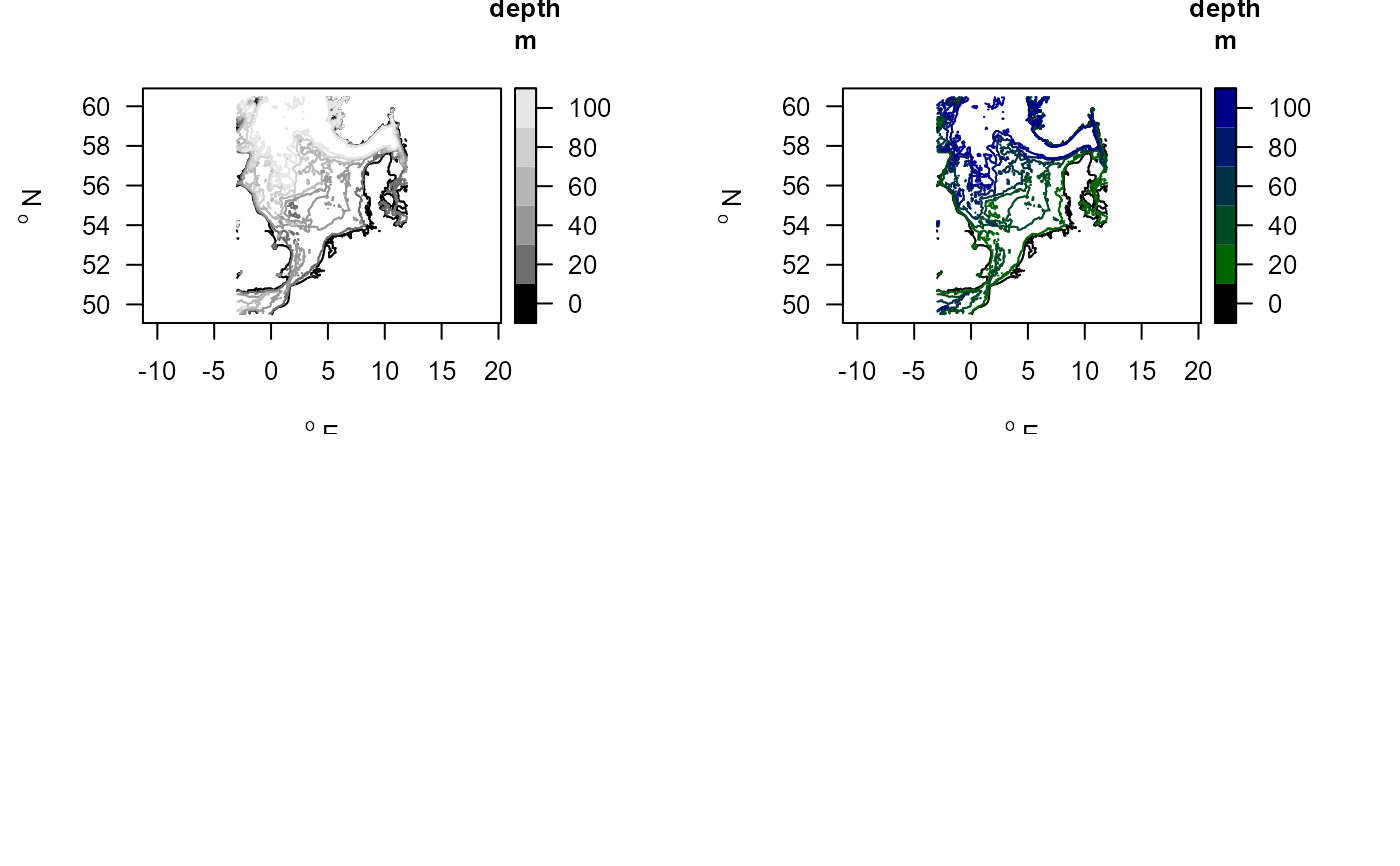
##-----------------------------------------------------
## Show the depth contours
##-----------------------------------------------------
map_key(contours = NSBS$contours,
draw.levels = TRUE, key.levels = TRUE)
# Use a different color scheme
collev <- function(n)
c("black", ramp.col(col = c("darkgreen", "darkblue"),
n = n-1))
map_key(contours = NSBS$contours,
draw.levels = TRUE, col.levels = collev,
key.levels = TRUE)
##-----------------------------------------------------
## Fishing data
##-----------------------------------------------------
metadata(NSBS$sar)
#> $data
#> name description units
#> 1 sandy sandy sediment (based on high/low dimensional) or not -
#> 2 year year of the fishing -
#> 3 gear metier; TBB, OT: beam, otter trawl; DRB: dredge, SN: seine -
#> 4 sar annual swept area ratios for the surface (0-2cm) /yr
#> 5 gpd estimated gear penetration depths cm
#>
# Sum fishing per year, per station
NSBSfish <- tapply(X = NSBS$sar$sar,
INDEX = list(NSBS$sar$station, NSBS$sar$year),
FUN = sum)
matplot(x = as.double(colnames(NSBSfish)),
y = t(NSBSfish),
xlab = "year", ylab = "m2/m2/yr",
main = "fishing intensity NSBS stations",
type = "l", log= "y")
##-----------------------------------------------------
## Community mean weighted score for typological groups.
##-----------------------------------------------------
# Groups is in crisp format -> convert to fuzzy
Groups.fuz <- crisp2fuzzy(Groups[,c("taxon", "typology")])
head (Groups, n = 2)
#> taxon Functional.group typology description
#> 1 Nephrops norvegicus 11 Deep3D Deep 3D burrower
#> 2 Upogebia deltaura 11 Deep3D Deep 3D burrower
head (Groups.fuz, n = c(2, 5))
#> taxon typology_Deep3D typology_DeepTub typology_Epi3D
#> 1 Nephrops norvegicus 1 0 0
#> 2 Upogebia deltaura 1 0 0
#> typology_Foul
#> 1 0
#> 2 0
group.cwm <- get_trait_density(wide = NSwide,
trait = Groups.fuz,
scalewithvalue = TRUE)
head(group.cwm, n=c(3,4))
#> descriptor typology_Deep3D typology_DeepTub typology_Epi3D
#> 1 ICES002 0 0.00000000 0
#> 2 ICES003 0 0.00000000 0
#> 3 ICES004 0 0.06191872 0
summary(group.cwm)
#> descriptor typology_Deep3D typology_DeepTub typology_Epi3D
#> Length :234 Min. :0.00000 Min. :0.00000 Min. :0.00000
#> N.unique :234 1st Qu.:0.00000 1st Qu.:0.01365 1st Qu.:0.00000
#> N.blank : 0 Median :0.00000 Median :0.05694 Median :0.00000
#> Min.nchar: 7 Mean :0.00303 Mean :0.10945 Mean :0.00147
#> Max.nchar: 7 3rd Qu.:0.00000 3rd Qu.:0.14237 3rd Qu.:0.00000
#> Max. :0.07873 Max. :0.86668 Max. :0.13739
#> typology_Foul typology_MajBiot typology_MinBiot typology_Neutral
#> Min. :0.000000 Min. :0.00000 Min. :0.00000 Min. :0.000000
#> 1st Qu.:0.000000 1st Qu.:0.06253 1st Qu.:0.04029 1st Qu.:0.000000
#> Median :0.003142 Median :0.11540 Median :0.07770 Median :0.000000
#> Mean :0.051520 Mean :0.13321 Mean :0.10534 Mean :0.003535
#> 3rd Qu.:0.023905 3rd Qu.:0.17352 3rd Qu.:0.13164 3rd Qu.:0.000000
#> Max. :1.000000 Max. :0.55688 Max. :0.62949 Max. :0.094942
#> typology_SesBiot typology_ShalShel typology_SmalTub typology_SurfDiff
#> Min. :0.00000 Min. :0.00000 Min. :0.00000 Min. :0.00000
#> 1st Qu.:0.01020 1st Qu.:0.02826 1st Qu.:0.03659 1st Qu.:0.09536
#> Median :0.07073 Median :0.08966 Median :0.07601 Median :0.17046
#> Mean :0.13557 Mean :0.12035 Mean :0.11163 Mean :0.22490
#> 3rd Qu.:0.23378 3rd Qu.:0.17512 3rd Qu.:0.16814 3rd Qu.:0.31458
#> Max. :0.74574 Max. :0.76394 Max. :0.47913 Max. :0.85365
##-----------------------------------------------------
## Show the depth contours
##-----------------------------------------------------
map_key(contours = NSBS$contours,
draw.levels = TRUE, key.levels = TRUE)
# Use a different color scheme
collev <- function(n)
c("black", ramp.col(col = c("darkgreen", "darkblue"),
n = n-1))
map_key(contours = NSBS$contours,
draw.levels = TRUE, col.levels = collev,
key.levels = TRUE)
##-----------------------------------------------------
## Fishing data
##-----------------------------------------------------
metadata(NSBS$sar)
#> $data
#> name description units
#> 1 sandy sandy sediment (based on high/low dimensional) or not -
#> 2 year year of the fishing -
#> 3 gear metier; TBB, OT: beam, otter trawl; DRB: dredge, SN: seine -
#> 4 sar annual swept area ratios for the surface (0-2cm) /yr
#> 5 gpd estimated gear penetration depths cm
#>
# Sum fishing per year, per station
NSBSfish <- tapply(X = NSBS$sar$sar,
INDEX = list(NSBS$sar$station, NSBS$sar$year),
FUN = sum)
matplot(x = as.double(colnames(NSBSfish)),
y = t(NSBSfish),
xlab = "year", ylab = "m2/m2/yr",
main = "fishing intensity NSBS stations",
type = "l", log= "y")