Simple plotting function for trait or density data
BtraitMap.Rdmap_key: plots contourlines of the dataset with colored data as points superimposed; a colorkey explains the colors
map_legend: plots contourlines of the dataset with colored data superimposed; point size depends on data value; a legend explains the colors and sizes
map_MWTL and map_NSBS are convenience functions for plotting the MWTL and NSBS data sets.
map_key (x = NULL, y = NULL, colvar = NULL,
         main = NULL, col = NULL, lwd = 1,
         colkey = list(), xlim = NULL, ylim = NULL, clim = NULL,
         contours = NULL, draw.levels = FALSE, col.levels = "black",
         by.levels=1, key.levels = FALSE, lwd.levels = 1, axes = TRUE,
         frame.plot = TRUE, asp = NULL, NApch = 43, ...)
map_legend (x = NULL, y = NULL, colvar = NULL,
         main = NULL, col = NULL, lwd = 1,
         legend = list(), xlim = NULL, ylim = NULL, clim = NULL,
         scale = "simple", pch = 18, cex = 3, cex.min = cex/20,
         contours = NULL, draw.levels = FALSE, col.levels = "black",
         by.levels=1, key.levels = FALSE, lwd.levels = 1, axes = TRUE,
         frame.plot = TRUE, asp = NULL, NApch = 43, NAtext = "NA", ...)

map_MWTL(x = NULL, y = NULL, colvar = NULL,
         draw.levels = TRUE, type = "key", ...)

map_NSBS(x = NULL, y = NULL, colvar = NULL,
         draw.levels = TRUE, type = "key", ...)
Arguments
- x, y
coordinates of the points to plot.
- colvar
color variable.
- col
The colors used for the color variable. A vector; the default is
jet.col(100).- colkey
specifications for the color key. See colkey.
- legend
specifications for the legend. Arguments as passed to legend. Also allowed are
side,cex,parsthat will be passed to legend.plt as legend.side, legend.cex and legend.pars respectively.- main
title of the plot.
- asp
aspect ratio of the plot. If
NULL, it will be estimated from the mean of the y-values, assuming these are latitudes.- xlim, ylim
ranges of the plot. When asp=NULL, the ranges will be only approximate, as the actual ranges are tuned by the aspect ratio, which is estimated from y.
- clim
range of the color variable values.
- scale
how to scale the size of the points, one of "simple", "abs" or "none", for scaling with the value, the absolute value or no scaling respectively.
- pch
the type of points to use; one value. If scale = "abs", a vector with two pch numbers is also allowed, first for the positive values, second pch for the negative values.
- lwd
the line width of the points to use; one value.
- cex, cex.min
maximum and minimum value of the pch size - cex.min will be ignored if scale = "none".
- contours
A list with
x,y, andzthat specifies the contours. Usually,zis the water depth.- draw.levels
Whether or not the depth levels should be added; if
FALSEonly contour levels that are >= 0 will be added.- col.levels
Colors of the depth levels (only applicable if
draw.levels=TRUE); the default is to have grey colors. Also allowed is a function that takes as input the number of colors - see last example.- by.levels
if levels need to be represented with less detail, set by.levels>1. This will speed up plotting. Only effective if contours is passed.
- lwd.levels
The line width of the depth contour lines.
- key.levels
Whether to add a color key with the depth levels; only applicable if
draw.levels=TRUE). This can be TRUE or FALSE, or a list that specifies the color key (see colkey).- axes, frame.plot
arguments to the main plotting function (that opens a window).
- ...
additional arguments passed to - for map_key- the plot function *points2D*, e.g. the type of symbol to use (pch, cex, ...), or whether to use log-transformed color variables (log="c").
- type
either "key" of "legend", so as to calle map_key or map_legend.
- NApch, NAtext
pch of the NA colvar, and the text in the legend. Note that, if pch is numeric, then also NApch should be numeric; NApch = 43 will draw a "+"","
Value
returns nothing
Note
These are simple plotting functions, and there may be better alternatives around.
If asp=NULL, then, to scale the x- and y-axis, the aspect ratio is estimated as: asp = 1/ cos((mean(ylim) * pi)/180).
Examples
## MWTL data
MWTLabiotics <- merge(MWTL$stations, MWTL$abiotics)
# =========================================
# 4 times the same data plotted
# =========================================
par (mfrow=c(2,2))
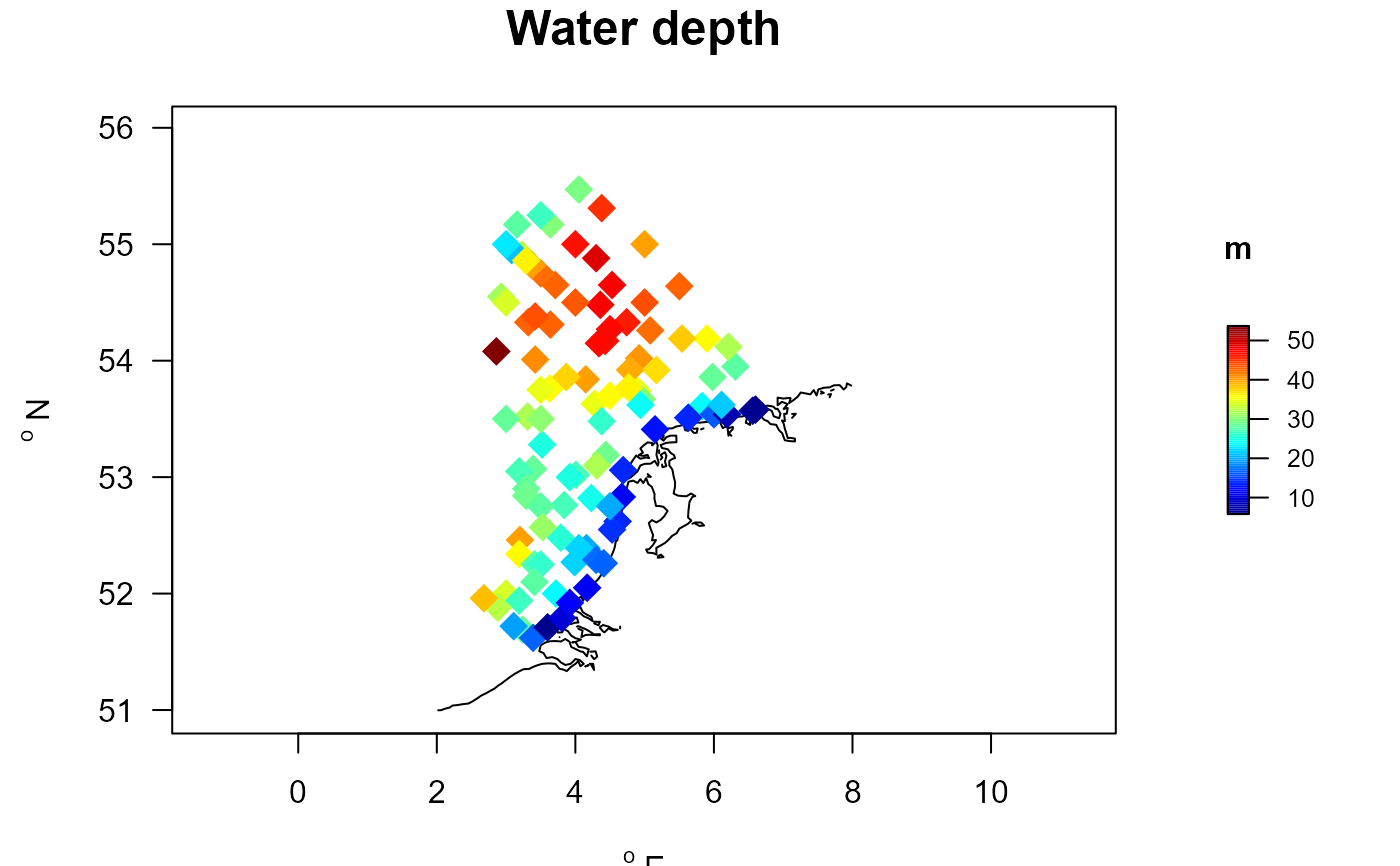
with (MWTLabiotics,
map_key(x, y, colvar = depth,
contours = MWTL$contours,
clab = "m", main = "Water depth",
pch = 18, cex = 2))
with (MWTLabiotics,
map_MWTL(x, y, colvar = depth,
clab = "m", main = "Water depth",
pch = 18, cex = 2))
with (MWTLabiotics,
map_legend(x, y, colvar = depth,
contours = MWTL$contours,
clab = "m", main = "Water depth",
pch = 18, cex = 2))
with (MWTLabiotics,
map_MWTL(x, y, colvar = depth,
clab = "m", main = "Water depth",
type = "legend", pch = 18, cex = 2))
 # =========================================
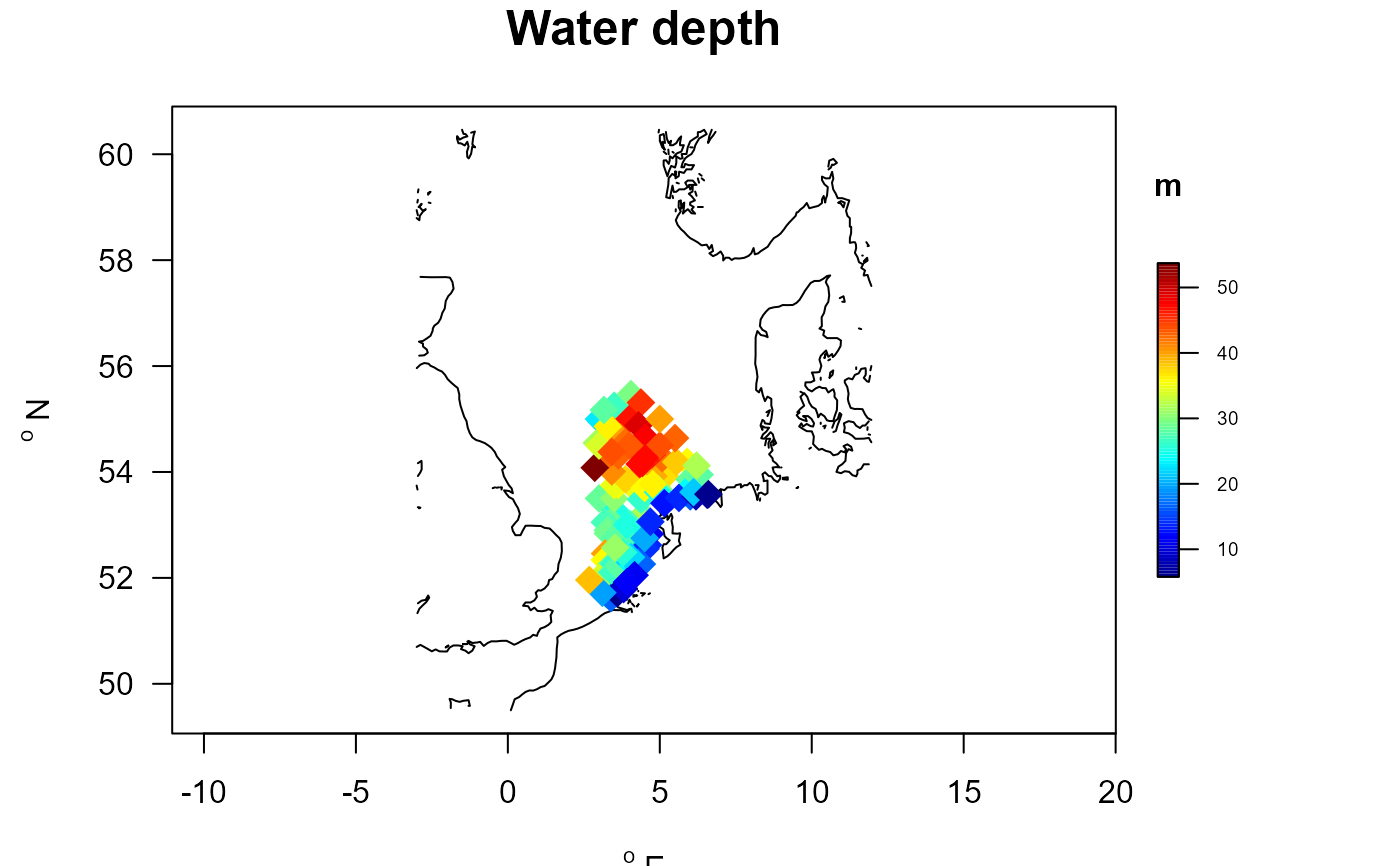
# Change the colorkey and the contours
# =========================================
with (MWTLabiotics,
map_key(x, y, colvar = depth, contours = NSBS$contours,
clab = "m", main = "Water depth",
colkey = list(dist = -0.05, length = 0.5,
width = 0.5, cex.axis = 0.6),
pch = 18, cex=2))
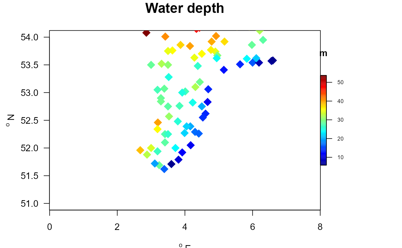
# zoom in on an area (not full control due to the overruling aspect ratio)
with (MWTLabiotics,
map_key(x, y , colvar = depth,
clab = "m", main = "Water depth",
ylim = c(51, 54), xlim = c(3,5),
colkey = list(dist = -0.08, length = 0.5,
width = 0.5, cex.axis = 0.6),
pch = 18, cex = 2))
#> Warning: no non-missing arguments to min; returning Inf
#> Warning: no non-missing arguments to max; returning -Inf
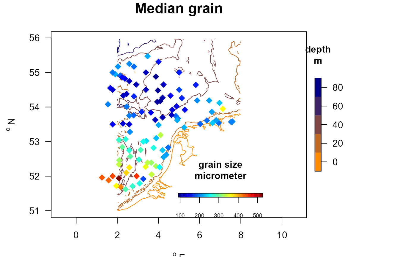
# adding also the contours
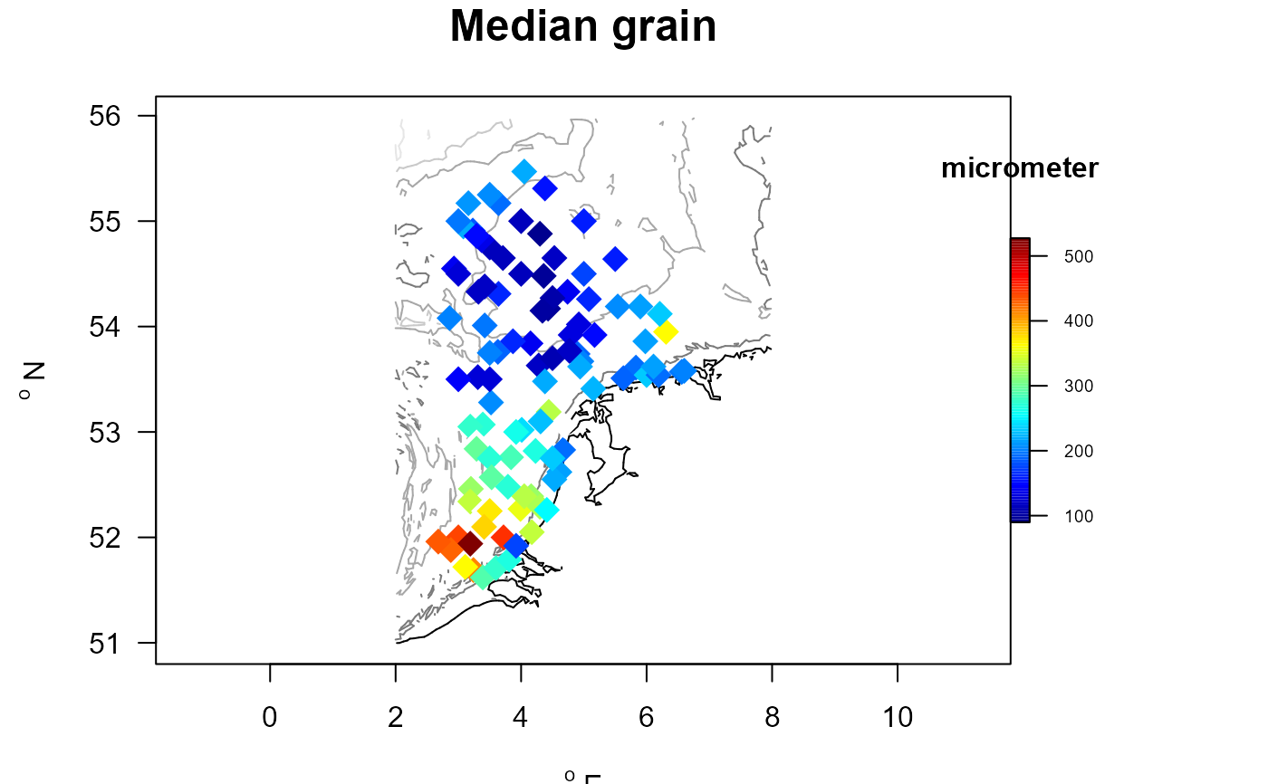
with (MWTLabiotics,
map_key(x, y, colvar = D50, contours = MWTL$contours,
clab = "micrometer", main = "Median grain",
draw.levels = TRUE,
colkey = list(dist = -0.08, length = 0.5,
width = 0.5, cex.axis = 0.6),
pch = 18, cex = 2))
# adding also the contours with color key
# note: - main color key then positioned elsewhere (side=1)
# Use a different color scheme
collev <- function(n)
ramp.col(col = c("darkorange", "darkblue"), n = n)
# Change the appearance of the colorkey for levels:
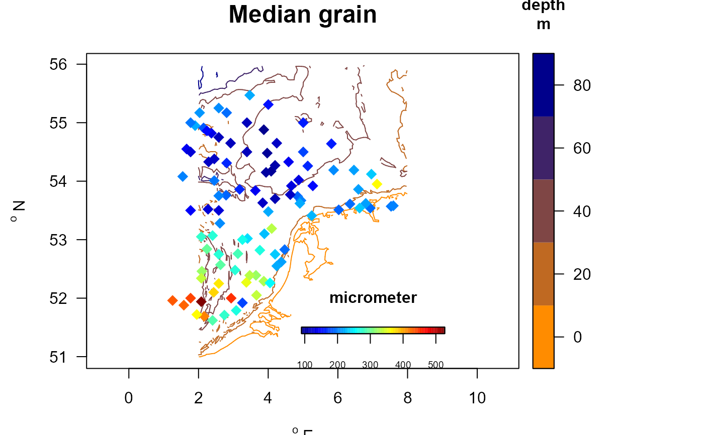
with (MWTLabiotics,
map_key(x, y, colvar = D50, contours=MWTL$contours,
clab = c("grain size", "micrometer"), main = "Median grain",
draw.levels = TRUE, key.levels = list(length = 0.5, width = 0.5),
col.levels = collev,
colkey = list(side = 1, dist = -0.08, length = 0.25,
width = 0.5, cex.axis = 0.6),
pch = 18, cex = 1.5))
# =========================================
# Change the colorkey and the contours
# =========================================
with (MWTLabiotics,
map_key(x, y, colvar = depth, contours = NSBS$contours,
clab = "m", main = "Water depth",
colkey = list(dist = -0.05, length = 0.5,
width = 0.5, cex.axis = 0.6),
pch = 18, cex=2))
# zoom in on an area (not full control due to the overruling aspect ratio)
with (MWTLabiotics,
map_key(x, y , colvar = depth,
clab = "m", main = "Water depth",
ylim = c(51, 54), xlim = c(3,5),
colkey = list(dist = -0.08, length = 0.5,
width = 0.5, cex.axis = 0.6),
pch = 18, cex = 2))
#> Warning: no non-missing arguments to min; returning Inf
#> Warning: no non-missing arguments to max; returning -Inf
# adding also the contours
with (MWTLabiotics,
map_key(x, y, colvar = D50, contours = MWTL$contours,
clab = "micrometer", main = "Median grain",
draw.levels = TRUE,
colkey = list(dist = -0.08, length = 0.5,
width = 0.5, cex.axis = 0.6),
pch = 18, cex = 2))
# adding also the contours with color key
# note: - main color key then positioned elsewhere (side=1)
# Use a different color scheme
collev <- function(n)
ramp.col(col = c("darkorange", "darkblue"), n = n)
# Change the appearance of the colorkey for levels:
with (MWTLabiotics,
map_key(x, y, colvar = D50, contours=MWTL$contours,
clab = c("grain size", "micrometer"), main = "Median grain",
draw.levels = TRUE, key.levels = list(length = 0.5, width = 0.5),
col.levels = collev,
colkey = list(side = 1, dist = -0.08, length = 0.25,
width = 0.5, cex.axis = 0.6),
pch = 18, cex = 1.5))
 # =========================================
# Show the depth contours only
# =========================================
map_key(contours = NSBS$contours,
draw.levels = TRUE, key.levels = TRUE, col.levels = collev)
# less detail
map_key(contours = NSBS$contours,
draw.levels = TRUE, key.levels = FALSE, by.levels = 10)
# depth contours with station postions
with (MWTLabiotics,
map_legend(x, y, colvar = rep(NA, times = length(x)),
contours = MWTL$contours, draw.levels = TRUE,
main = "MWTL", NApch = "+", NAtext = "station positions",
legend = list(side=0, x = "bottomright")))
#------------------------------
# log-transformed color variables
#------------------------------
# average densities of Abra alba in the MWTL data.
A.alba <- get_density(data = MWTL$density,
descriptor = station,
averageOver = year,
taxon = taxon,
value = density,
subset = taxon == "Abra alba")
# add positions of stations
# all.x=TRUE: also stations without A.alba are selected
# the NAs are converted to 0
A.alba <- merge(MWTL$stations, A.alba,
by = 1, all.x = TRUE)
A.alba$value[which(is.na(A.alba$density))] <- 0
# plot with density values log-transfored
# 0-values will be transformed to NAs in map_key;
# we set the NA color="grey"
par(mfrow = c(2, 2))
# =========================================
# Show the depth contours only
# =========================================
map_key(contours = NSBS$contours,
draw.levels = TRUE, key.levels = TRUE, col.levels = collev)
# less detail
map_key(contours = NSBS$contours,
draw.levels = TRUE, key.levels = FALSE, by.levels = 10)
# depth contours with station postions
with (MWTLabiotics,
map_legend(x, y, colvar = rep(NA, times = length(x)),
contours = MWTL$contours, draw.levels = TRUE,
main = "MWTL", NApch = "+", NAtext = "station positions",
legend = list(side=0, x = "bottomright")))
#------------------------------
# log-transformed color variables
#------------------------------
# average densities of Abra alba in the MWTL data.
A.alba <- get_density(data = MWTL$density,
descriptor = station,
averageOver = year,
taxon = taxon,
value = density,
subset = taxon == "Abra alba")
# add positions of stations
# all.x=TRUE: also stations without A.alba are selected
# the NAs are converted to 0
A.alba <- merge(MWTL$stations, A.alba,
by = 1, all.x = TRUE)
A.alba$value[which(is.na(A.alba$density))] <- 0
# plot with density values log-transfored
# 0-values will be transformed to NAs in map_key;
# we set the NA color="grey"
par(mfrow = c(2, 2))
 map_key (A.alba$x, A.alba$y, colvar = A.alba$density,
main = "Abra alba",
contours = MWTL$contours,
cex = 2, pch = 18)
map_legend(A.alba$x, A.alba$y, colvar = A.alba$density,
main = "Abra alba",
contours = MWTL$contours,
NAtext = "absent",
cex = 4, pch = 16)
# log transformation converts 0 values into NAs
map_key (A.alba$x, A.alba$y, colvar = A.alba$density,
main = "Abra alba",
contours = MWTL$contours, NAcol = "grey", log = "c",
cex = 2, pch = 18)
map_legend(A.alba$x, A.alba$y, colvar = A.alba$density,
main = "Abra alba",
contours = MWTL$contours, NAtext = "absent",
log = "c", cex = 4, pch = 16)
map_key (A.alba$x, A.alba$y, colvar = A.alba$density,
main = "Abra alba",
contours = MWTL$contours,
cex = 2, pch = 18)
map_legend(A.alba$x, A.alba$y, colvar = A.alba$density,
main = "Abra alba",
contours = MWTL$contours,
NAtext = "absent",
cex = 4, pch = 16)
# log transformation converts 0 values into NAs
map_key (A.alba$x, A.alba$y, colvar = A.alba$density,
main = "Abra alba",
contours = MWTL$contours, NAcol = "grey", log = "c",
cex = 2, pch = 18)
map_legend(A.alba$x, A.alba$y, colvar = A.alba$density,
main = "Abra alba",
contours = MWTL$contours, NAtext = "absent",
log = "c", cex = 4, pch = 16)
 A.alba$value[A.alba$value==0] <- NA
map_legend(A.alba$x, A.alba$y, colvar = A.alba$density,
main = "Abra alba",
contours = MWTL$contours, NAtext = "absent",
cex = 4, pch = 16)
#------------------------------
# mappng with Legend
#------------------------------
DD <- merge(MWTL$stations, MWTL$abiotics)
with(DD, map_legend(x, y, colvar = D50,
contours = MWTL$contours))
with(DD, map_legend(x, y, colvar = seq(-1, 1, len = nrow(DD)),
contours = MWTL$contours))
with(DD, map_legend(x, y, colvar = seq(-1, 1, len = nrow(DD)),
scale = "abs",
contours = MWTL$contours,
pch = c(15, 22)))
A.alba$value[A.alba$value==0] <- NA
map_legend(A.alba$x, A.alba$y, colvar = A.alba$density,
main = "Abra alba",
contours = MWTL$contours, NAtext = "absent",
cex = 4, pch = 16)
#------------------------------
# mappng with Legend
#------------------------------
DD <- merge(MWTL$stations, MWTL$abiotics)
with(DD, map_legend(x, y, colvar = D50,
contours = MWTL$contours))
with(DD, map_legend(x, y, colvar = seq(-1, 1, len = nrow(DD)),
contours = MWTL$contours))
with(DD, map_legend(x, y, colvar = seq(-1, 1, len = nrow(DD)),
scale = "abs",
contours = MWTL$contours,
pch = c(15, 22)))
 with(DD, map_legend(x, y, colvar = seq(-1, 1, len = nrow(DD)),
scale = "abs",
contours = MWTL$contours, clab = "TRY",
legend = list(title.col="red"),
pch = 22, lwd = 2))
with(DD, map_legend(x, y, colvar = seq(-1, 1, len = nrow(DD)),
scale = "abs",
contours = MWTL$contours, clab = "TRY",
legend = list(title.col="red"),
pch = 22, lwd = 2))