The benthic fauna data from the Dutch part of the Northsea, including abiotic conditions.
MWTLdensitydata.RdThe MWTL Northsea macrobenthos data (1995 - 2018)
The dataset contains:
Macrofauna species density and biomass (MWTL$density)
abiotic conditions (MWTL$abiotics), station types (MWTL$types), sediment composition (MWTL$sediment) and station positions (MWTL$stations)
MWTL$contours: depth contourlines for mapping.
MWTL$fishing: species trait values that can be used to estimate fishing parameters.
MWTL$sar: station-specific fishing intensities.
data(MWTL)Format
==================
**MWTL$density**:
This is the main Northsea MWTL benthos data set, containing species
information for 103 stations sampled on a yearly basis from 1995 till 2010,
after which sampling was less frequent: in 2012, 2015 and 2018.
The data, in long format, are in a data.frame with the following columns:
station, the MWTL station name (details in MWTL$stations).date, the sampling date. Note, this is a string; it can be converted to POSIXct by:as.POSIXct(MWTL$density$date, format='%d-%m-%Y'). The year can be extracted as1900+as.POSIXlt(MWTL$density$date, format='%d-%m-%Y')$year.year, the year of samplingtaxon, the taxon name to be used (usually species); this has been derived from the original taxon in the MWTL data as follows: The original taxon e.g. species is kept, if a minimum of 90% of individual organisms of this taxon are at the species level, genus otherwise, if not family etc. The taxon name was checked against the WoRMS database (details in datasetTaxonomy).density, the number of individuals per m2.biomass, the total biomass per m2, in AFDW/m2 (ash-free dry weight)taxon.original, the original taxon name in the data set (see details).
=========================================
**MWTL$abiotics**:
the abiotic conditions of sampling stations.
MWTL$abiotics is a data.frame with the following columns:
station, the NSBS station name
depth, water depth, [m]
D50, Median grain size, [micrometer]
mud, mud content of sediment (<63 um), fraction, [-]
sand, sand fraction (64 -2000 um), [-]
gravel, gravel fraction (>2000 um), [-]
salinity, salinity
porosity, volumetric water content, [-]
permeability, sediment permeability, [m2]
POC, particulate organic C in sediment, [percent]
TN, total N in sediment, [percent]
surfaceCarbon, particulate organic C in upper cm, [percent]
surfaceNitrogen, total N in upper cm, [percent]
orbitalVelMean, mean orbital velocity, [m/s]
orbitalVelMax, maximal orbital velocity, [m/s]
tidalVelMean, mean tidal velocity, [m/s]
tidalVelMax, maximal tidal velocity, [m/s]
bedstress, bed shear stress, [Pa]
EUNIScode, EUNIScode, [-]
DRB, swept area ratio for dredge, [m2/m2/year]
OT, swept area ratio for otter trawl, [m2/m2/year]
SN, swept area ratio for seines, [m2/m2/year]
TBB, swept area ratio for beam trawl, [m2/m2/year]
sar, total swept area ratio , DRB +OT +SN +TBB, [m2/m2/year]
subsar, swept area ratio (fisheries) > 2cm, [m2/m2/year]
gpd, gear penetration depth, [cm]
The fishing data (sar, subsar, gpd) were derived from ICES upon request by OSPAR.
They are averaged over (2009-2018). See also MWTL$sar.
==================
**MWTL$fishing**:
species trait values that can be used to estimate fishing parameters.
==================
**MWTL$types**:
the abiotic conditions of sampling stations, typologies
MWTL$types categorizes the stations into a number of types:
station, the MWTL station name.
depth (m)
Very shallow: < 10,
Shallow: [10; 20[,
Intermediate: [20; 30[,
Deep: [30; 40[,
Very deep: >= 40
current (m/s):
Very low: < 0.15,
Low: [0.15; 0.20[,
Intermediate: [0.20; 0.25[,
High: [0.25; 0.30[,
Very high: >= 0.30
The numbers are Monthly median values, in meters per second averaged from 1996 to 2008
wave energy (Pa):
Very low: < 0.5,
Low: [0.5; 1.0[,
Intermediate: [1.0; 1.5[,
High: [1.5; 2.0[,
Very high: >= 2.0
; the data are monthly median values in pascals averaged from 1996 to 2008.
stratification
PM : Permanently mixed
FI : Freshwater influence
IS : Intermittently stratified
SS : Seasonally stratified
TR : Transitional
sediment
Muddy includes Mud, Sandy mud, Sandy and slightly gravely mud, Muddy sand;
Sandy means only Sand;
Coarse includes: Gravel and muddy sand, Slightly gravely sand, Gravely sand, Sandy gravel, Gravel and stone;
Mixed includes Gravely and slightly muddy sand,
where clay <8 um, silt: 8-63, very fine sand: 62-125, fine sand: 125-250, medium sand: 250-500, coarse sand: 500-1000, very coarse sand: 1000-2000, gravel: >2000 um (micrometer).
BPI_xx Benthic Terrain Classification parameters, bathymetric position index
dynamics
L: low
H: high
area
DOG: Doggersbank
OYS: Oystergrounds
OFF: Offshore
COA: Coastal zone
==================
**MWTL$stations**:
The positions of the different stations, in WGS84 format
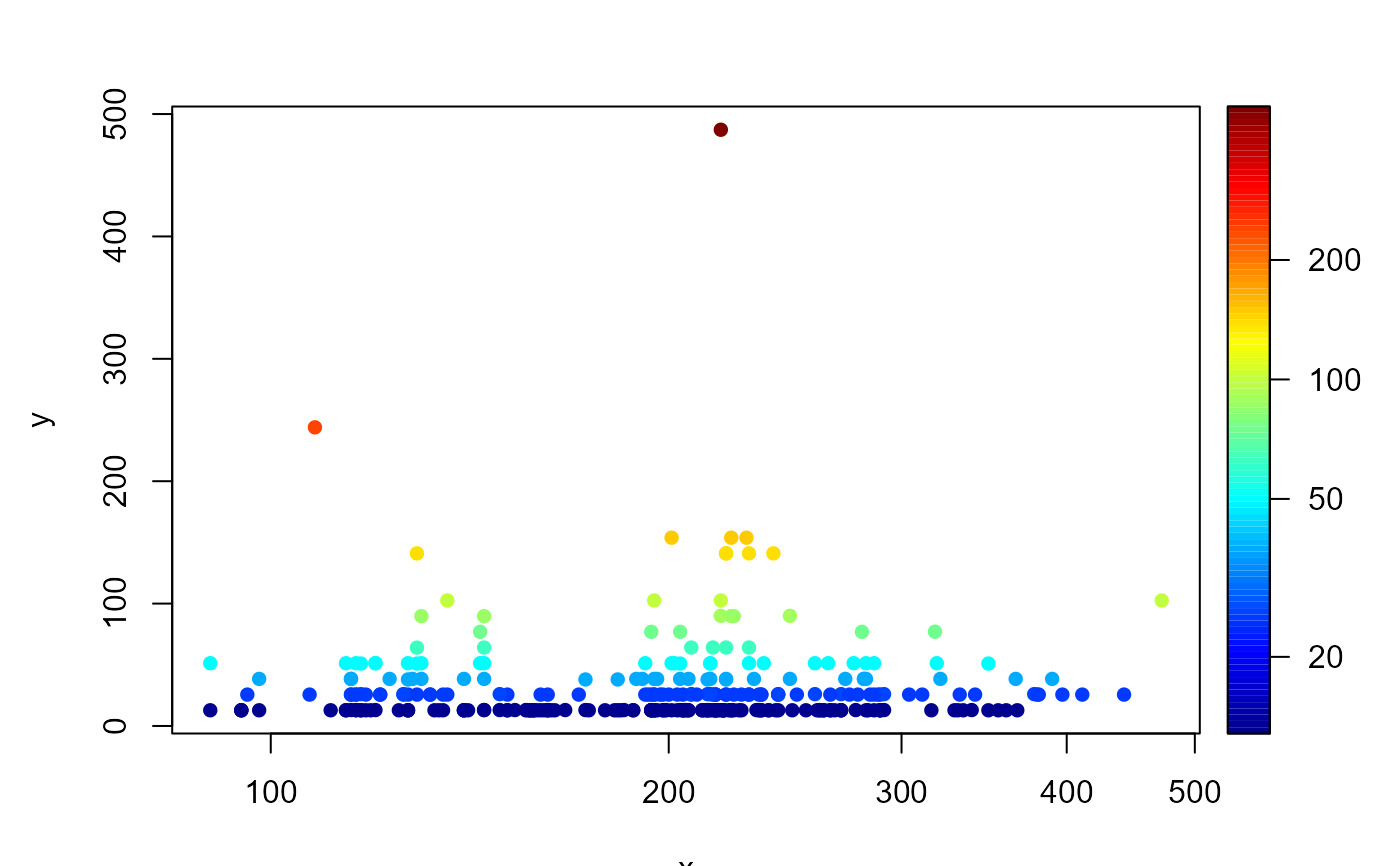
station, the MWTL station name.
x, degrees longitude
y, degrees latitude
==================
**MWTL$sediment**:
records the sediment characteristics (median grain size and silt content)
for the different stations and years.
The data for "BREEVTN11" "BREEVTN16" "WADDKT05" are missing.
This is a data.frame with:
station, the MWTL station name.
year, the sampling year.
D50, the median grain size of the sediment, in micrometer
silt, the silt and clay content (< 63 micrometer), in percentage
De sediment grainsize was determined by laserdiffraction using a Malvern Mastersizer. Values denote weight percentages dryweight of the total sediment sample, where big shells and large animals were removed.
==================
**MWTL$contours**:
The data for plotting the depth contours in the area.
The contourlines (x-, y) were derived from GEBCO high-resolution bathymetry,
by using the contourLines R-function.
The data set contains:
x: longitude, in [dgE]
y: latitude, in [dgN]
z: the corresponding depths, [m]
==================
**MWTL$sar**:
Fishing intensity data for the MWTL stations, origin: ICES upon request by OSPAR. The NSBS stations nearest to the ICES data were selected.
A data.frame that contains:
station, the NSBS station name
year: the fishing year
gear: metier; TBB, OT: beam, otter trawl; DRB: dredge, SN: seine.
sar: annual swept area ratios (m2/m2/yr) for the surface (0-2cm).
subsar: annual swept area ratios (m2/m2/yr) for the subsurface (>2cm).
gpd: estimated gear penetration depths ([cm]), based on metier
Note
The dataset **Taxonomy**:
contains taxonomic information of the original and adjusted taxon in MWTL$density,
as derived from the World Register of Marine Species (WoRMS), using R-package worrms.
Details
The *macrobenthos data* of the Northsea (MWTL) are commissioned by the "Ministerie van Infrastructuur en Milieu, Rijkswaterstaat Centrale Informatievoorziening (RWS, CIV)".
MWTL stands for Monitoring Waterstaatkundige Toestand des Lands (dutch).
Sediment was sampled with a Reineck Boxcorer (0,078 m2). Macrofauna sieved on a 1 mm mesh. All animals determined, except when too much residue or organisms, in which case samples were subsampled, so that for molluscs and crustaceans at least 100 individuals, and for polychaetes at least 150 individuals were determined.
Biomass was determined as ash-free dryweight: individuals were dried for >48 hours at 65 dgC, and then cooled in an exsiccator for at least 30 minutes and weighed (precision 0,01 mg), determining their dryweight. Then they were ashed in an oven at 530 dgC (2,5, 4 or 8 hour, depending on the size of organisms). Following ashing, they were weighed, after cooling for at least 45 minutes in an exsiccator. Bivalvia and Gastropoda =7 mm were ashed without shell, but when smaller than 7 mm the shell was not removed.
AFDW = (dryweight + weight cup) ? (ash weight + weight cup).
=====================================================================
The *fishing data* (in abiotics and sar) were derived from ICES upon request by OSPAR.
They are averaged over (2009-2018).
The metiers are Aggregated into beam trawl (TBB), dredge (DRB), demersal seine (SN), and otter trawl (OT), based on the metier layers: OT_CRU, OT_DMF, OT_MIX, OT_MIX_CRU, OT_MIX_DMF_BEN, OT_MIX_DMF_PEL, OT_MIX_CRU_DMF, OT_SPF, TBB_CRU, TBB_DMF, TBB_MOL, DRB_MOL, SDN_DMF, SSC_DMF
The gear penetration depths used were:
in sand: 3.5, 1.1, 1.1, 1.9 cm for DRB, OT, SN, TBB respectively
in mud : 5.4, 2.0, 2.0, 3.2 cm for DRB, OT, SN, TBB respectively
The sediment was assumed to be "mud" when the type "sediment" was "Muddy"
References
The taxonomic information was created using the worrms package:
Chamberlain S, Vanhoorne. B (2023). worrms: World Register of Marine Species (WoRMS) Client_. R package version 0.4.3, <https://CRAN.R-project.org/package=worrms>.
The MWTL data are described in:
L. Leewis, E.C. Verduin, R. Stolk ; Eurofins AquaSense Macrozoobenthosonderzoek in de Rijkswateren met boxcorer, jaarrapportage MWTL 2015 : waterlichaam: Noordzee Publicatiedatum: 31-03-201775 p. Projectnummer Eurofins AquaSense: J00002105. Revisie 2, In opdracht van Ministerie van Infrastructuur en Milieu, Rijkswaterstaat Centrale Informatievoorziening (RWS, CIV)
The fishing data were derived from:
ICES Technical Service, Greater North Sea and Celtic Seas Ecoregions, 29 August 2018 sr.2018.14 Version 2: 22 January 2019 https://doi.org/10.17895/ices.pub.4508 OSPAR request on the production of spatial data layers of fishing intensity/pressure.
See also
map_key for plotting.
Traits_nioz for the trait datasets.
get_density for functions operating on these data.
long2wide for functions changing the appearance on these data.
get_Db_index for extracting bioturbation and bioirrigation indices.
Examples
##-----------------------------------------------------
## Show contents of the data set
##-----------------------------------------------------
metadata(MWTL$sediment)
#> name description units
#> 1 D50 median grain size, in micrometer micrometer
#> 2 Silt Silt+Clay fraction (< 63 micrometer) in % %
metadata(MWTL$abiotics)
#> name description units
#> 1 depth water depth m
#> 2 D50 Median grain size micrometer
#> 3 mud mud fraction (<63 um) -
#> 4 sand sand fraction (64 -2000 um) -
#> 5 gravel gravel fraction (>2000 um) -
#> 6 salinity salinity
#> 7 porosity volumetric water content -
#> 8 permeability permeability m2
#> 9 POC particulate organic C in sediment %
#> 10 TN total N in sediment %
#> 11 surfaceCarbon particulate organic C in upper cm %
#> 12 surfaceNitrogen total N in upper cm %
#> 13 orbitalVelMean mean orbital velocity m/s
#> 14 orbitalVelMax maximal orbital velocity m/s
#> 15 tidalVelMean mean tidal velocity m/s
#> 16 tidalVelMax maximal tidal velocity m/s
#> 17 bedstress bed shear stress Pa
#> 18 EUNIScode EUNIScode -
#> 19 DRB swept area ratio for dredge m2/m2/year
#> 20 OT swept area ratio for otter trawl m2/m2/year
#> 21 SN swept area ratio for seines m2/m2/year
#> 22 TBB swept area ratio for beam trawl m2/m2/year
#> 191 sar swept area ratio (fisheries), DRB +OT +SN +TBB m2/m2/year
#> 201 subsar swept area ratio (fisheries) > 2cm m2/m2/year
#> 211 gpd gear penetration depth cm
metadata(MWTL$types)
#> $stratification
#> [1] "PM=Permanently mixed, FI=Freshwater influence, IS=Intermittently stratified, SS=Seasonally stratified, TR=Transitional"
#>
#> $sediment
#> [1] "'Muddy'=[Mud, Sandy mud, Sandy and slightly gravely mud, Muddy sand]; 'Sandy'= [Sand]; 'Coarse'=[Gravel and muddy sand, Slightly gravely sand, Gravely sand, Sandy gravel, Gravel and stone]; 'Mixed' = [Gravely and slightly muddy sand], where 'clay'=[<8 um], 'silt'=[8-63], ' 'very fine sand'=[62-125], 'fine sand'=[125-250], 'medium sand'=[250-500], 'coarse sand'=[500-1000], 'very coarse sand'=[1000-2000], 'gravel'=[>2000 um] (micrometer)."
#>
#> $depth
#> [1] "'Very shallow'=[<10m]; 'Shallow'=[10; 20[; 'Intermediate'=[20; 30[; 'Deep'=[30; 40[; 'Very deep'=[>= 40m]"
#>
#> $current
#> [1] "'Very low'=[<0.15]; 'Low'=[0.15; 0.20[; 'Intermediate'=[0.20; 0.25[; 'High'=[0.25; 0.30[; 'Very high'=[>=0.30m/s]"
#>
#> $wave
#> [1] "Very low < 0.5; Low [0.5; 1.0[; Intermediate [1.0; 1.5[; High [1.5; 2.0[; Very high >= 2.0"
#>
#> $BPx
#> [1] "bathymetric position index derived from ship-borne multibeam swath acoustic data"
#>
#> $dynamics
#> [1] "L=low; H=high"
#>
#> $area
#> [1] "Coast (COA), Doggerbank (DOG), Offshore (OFF), Oystergrounds (OYS)"
#>
#> $group
#> [1] "derived from first part of station name"
#>
metadata(MWTL$density)
#> name description units
#> 1 station station name
#> 2 date sampling date, a string
#> 3 taxon taxon name, checked by worms, and adjusted
#> 4 density species total density individuals/m2
#> 5 biomass species total ash-free dry weight gAFDW/m2
#> 6 taxon.original original taxon name
metadata(MWTL$sar)
#> $data
#> name description units
#> 1 sandy sandy sediment (based on high/low dimensional) or not -
#> 2 year year of the fishing -
#> 3 gear metier; TBB, OT: beam, otter trawl; DRB: dredge, SN: seine -
#> 4 sar annual swept area ratios for the surface (0-2cm) /yr
#> 5 gpd estimated gear penetration depths cm
#>
##-----------------------------------------------------
## SPECIES data
##-----------------------------------------------------
head(MWTL$density)
#> station date year taxon density biomass
#> 1 BREEVTN02 27-06-1995 1995 Bathyporeia guilliamsoniana 14.6 0.0044
#> 2 BREEVTN02 27-06-1995 1995 Callianassa 58.5 1.3986
#> 3 BREEVTN02 27-06-1995 1995 Chaetozone setosa 14.6 0.0073
#> 4 BREEVTN02 27-06-1995 1995 Chamelea striatula 14.6 2.7738
#> 5 BREEVTN02 27-06-1995 1995 Echinocardium 43.9 0.0044
#> 6 BREEVTN02 27-06-1995 1995 Echinocardium 14.6 4.9435
#> taxon.original
#> 1 Bathyporeia guilliamsoniana
#> 2 Callianassa subterranea
#> 3 Chaetozone setosa
#> 4 Chamelea striatula
#> 5 Echinocardium
#> 6 Echinocardium cordatum
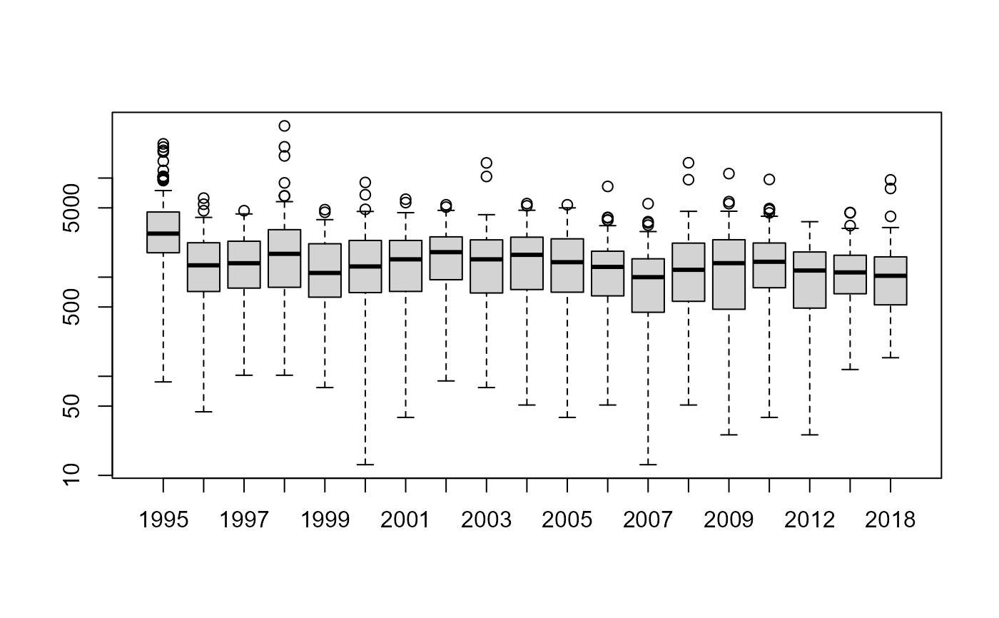
# The number of species per station (over all years)
Nspecies <- tapply(X = MWTL$density$taxon,
INDEX = MWTL$density$station,
FUN = function(x)length(unique(x)))
summary(Nspecies)
#> Min. 1st Qu. Median Mean 3rd Qu. Max.
#> 16.00 58.50 88.00 82.14 105.50 132.00
# Per year
Nspyear <- tapply(X = MWTL$density$taxon,
INDEX = list(MWTL$density$station, MWTL$density$year),
FUN = function(x)length(unique(x)))
colMeans(Nspyear, na.rm=TRUE)
#> 1995 1996 1997 1998 1999 2000 2001 2002
#> 24.07000 18.60606 21.00000 21.33000 20.46000 22.01000 22.39000 24.01000
#> 2003 2004 2005 2006 2007 2008 2009 2010
#> 22.14000 21.95000 21.00980 20.37000 18.24000 19.09000 18.88000 20.97000
#> 2012 2015 2018
#> 19.56000 20.30303 19.60204
# The number of times a species has been found
Nocc <- tapply(X = MWTL$density$station,
INDEX = MWTL$density$taxon,
FUN = length)
head(sort(Nocc, decreasing = TRUE)) #most often encountered taxa
#> Nephtys Magelona Nemertea Spiophanes bombyx
#> 2785 1760 1272 1198
#> Phoronis Echinocardium
#> 996 948
# total density
densyear <- tapply(X = MWTL$density$density,
INDEX = list(MWTL$density$station, MWTL$density$year),
FUN = sum)
boxplot(densyear, log="y")
 ##-----------------------------------------------------
## ABIOTICS data
##-----------------------------------------------------
summary(MWTL$abiotics)
#> station depth D50 mud
#> Length :103 Min. : 5.80 Min. : 90.0 Min. :0.00002
#> N.unique :103 1st Qu.:24.10 1st Qu.:148.4 1st Qu.:0.00100
#> N.blank : 0 Median :29.60 Median :205.1 Median :0.01105
#> Min.nchar: 7 Mean :30.37 Mean :222.6 Mean :0.05160
#> Max.nchar: 9 3rd Qu.:39.50 3rd Qu.:273.4 3rd Qu.:0.06319
#> Max. :53.70 Max. :527.1 Max. :0.34772
#> NAs :3
#> sand gravel salinity porosity
#> Min. :0.6523 Min. :0.0001033 Min. :27.63 Min. :0.3821
#> 1st Qu.:0.9368 1st Qu.:0.0001251 1st Qu.:32.91 1st Qu.:0.3955
#> Median :0.9889 Median :0.0001861 Median :34.30 Median :0.4056
#> Mean :0.9483 Mean :0.0010354 Mean :33.46 Mean :0.4158
#> 3rd Qu.:0.9990 3rd Qu.:0.0005031 3rd Qu.:34.53 3rd Qu.:0.4312
#> Max. :1.0000 Max. :0.0201886 Max. :34.77 Max. :0.5102
#>
#> permeability POC TN surfaceCarbon
#> Min. :4.759e-15 Min. :0.04682 Min. :0.03000 Min. :0.07304
#> 1st Qu.:9.380e-14 1st Qu.:0.16854 1st Qu.:0.03426 1st Qu.:0.26410
#> Median :3.882e-13 Median :0.22429 Median :0.03690 Median :0.34363
#> Mean :1.112e-12 Mean :0.27913 Mean :0.04310 Mean :0.42828
#> 3rd Qu.:1.030e-12 3rd Qu.:0.41189 3rd Qu.:0.04940 3rd Qu.:0.62366
#> Max. :1.530e-11 Max. :0.69416 Max. :0.08074 Max. :1.11217
#> NAs :1 NAs :1 NAs :1
#> surfaceNitrogen orbitalVelMean orbitalVelMax tidalVelMean
#> Min. :0.04522 Min. :0.02655 Min. :0.2493 Min. :0.1100
#> 1st Qu.:0.05343 1st Qu.:0.04995 1st Qu.:0.4157 1st Qu.:0.1569
#> Median :0.05742 Median :0.06651 Median :0.5075 Median :0.2261
#> Mean :0.06652 Mean :0.08495 Mean :0.5785 Mean :0.2408
#> 3rd Qu.:0.07421 3rd Qu.:0.08331 3rd Qu.:0.6041 3rd Qu.:0.2998
#> Max. :0.12846 Max. :0.77342 Max. :3.3570 Max. :0.4878
#> NAs :1
#> tidalVelMax bedstress EUNIScode DRB
#> Min. :0.2501 Min. :0.0500 Length :103 Min. :0.000e+00
#> 1st Qu.:0.3352 1st Qu.:0.1350 N.unique : 3 1st Qu.:0.000e+00
#> Median :0.4862 Median :0.3300 N.blank : 0 Median :0.000e+00
#> Mean :0.5128 Mean :0.4562 Min.nchar: 4 Mean :3.949e-06
#> 3rd Qu.:0.6432 3rd Qu.:0.6900 Max.nchar: 4 3rd Qu.:0.000e+00
#> Max. :0.9724 Max. :1.3950 Max. :2.253e-04
#> NAs :4
#> OT SN TBB sar
#> Min. :0.0006321 Min. :0.0003635 Min. : 0.002649 Min. : 0.08889
#> 1st Qu.:0.0314983 1st Qu.:0.0058540 1st Qu.: 0.283902 1st Qu.: 0.86787
#> Median :0.1809426 Median :0.0202822 Median : 0.887328 Median : 1.37972
#> Mean :0.5357584 Mean :0.1350345 Mean : 1.416668 Mean : 2.08746
#> 3rd Qu.:0.6711816 3rd Qu.:0.0747842 3rd Qu.: 1.364096 3rd Qu.: 2.31002
#> Max. :6.0618379 Max. :2.5017089 Max. :11.789892 Max. :11.81743
#>
#> subsar gpd
#> Min. :0.01176 Min. :1.120
#> 1st Qu.:0.36041 1st Qu.:1.550
#> Median :1.06005 Median :1.813
#> Mean :1.16446 Mean :1.801
#> 3rd Qu.:1.42023 3rd Qu.:1.896
#> Max. :6.21711 Max. :3.111
#>
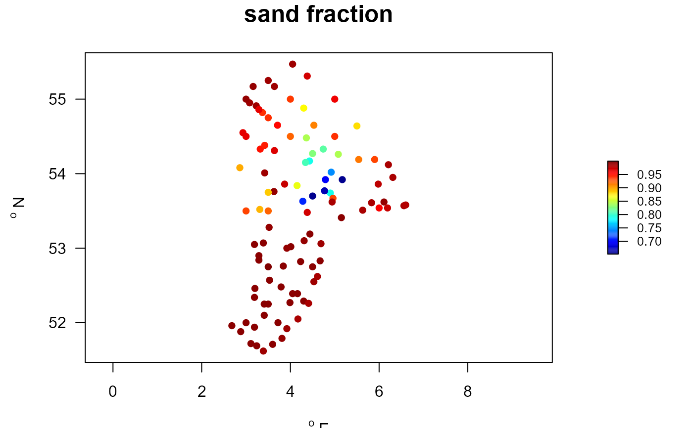
MWTLabiot <- merge(MWTL$stations, MWTL$abiotics)
with(MWTLabiot, map_key(x, y, colvar = sand,
main = "sand fraction",
pch = 16))
#> Warning: no non-missing arguments to min; returning Inf
#> Warning: no non-missing arguments to max; returning -Inf
##-----------------------------------------------------
## ABIOTICS data
##-----------------------------------------------------
summary(MWTL$abiotics)
#> station depth D50 mud
#> Length :103 Min. : 5.80 Min. : 90.0 Min. :0.00002
#> N.unique :103 1st Qu.:24.10 1st Qu.:148.4 1st Qu.:0.00100
#> N.blank : 0 Median :29.60 Median :205.1 Median :0.01105
#> Min.nchar: 7 Mean :30.37 Mean :222.6 Mean :0.05160
#> Max.nchar: 9 3rd Qu.:39.50 3rd Qu.:273.4 3rd Qu.:0.06319
#> Max. :53.70 Max. :527.1 Max. :0.34772
#> NAs :3
#> sand gravel salinity porosity
#> Min. :0.6523 Min. :0.0001033 Min. :27.63 Min. :0.3821
#> 1st Qu.:0.9368 1st Qu.:0.0001251 1st Qu.:32.91 1st Qu.:0.3955
#> Median :0.9889 Median :0.0001861 Median :34.30 Median :0.4056
#> Mean :0.9483 Mean :0.0010354 Mean :33.46 Mean :0.4158
#> 3rd Qu.:0.9990 3rd Qu.:0.0005031 3rd Qu.:34.53 3rd Qu.:0.4312
#> Max. :1.0000 Max. :0.0201886 Max. :34.77 Max. :0.5102
#>
#> permeability POC TN surfaceCarbon
#> Min. :4.759e-15 Min. :0.04682 Min. :0.03000 Min. :0.07304
#> 1st Qu.:9.380e-14 1st Qu.:0.16854 1st Qu.:0.03426 1st Qu.:0.26410
#> Median :3.882e-13 Median :0.22429 Median :0.03690 Median :0.34363
#> Mean :1.112e-12 Mean :0.27913 Mean :0.04310 Mean :0.42828
#> 3rd Qu.:1.030e-12 3rd Qu.:0.41189 3rd Qu.:0.04940 3rd Qu.:0.62366
#> Max. :1.530e-11 Max. :0.69416 Max. :0.08074 Max. :1.11217
#> NAs :1 NAs :1 NAs :1
#> surfaceNitrogen orbitalVelMean orbitalVelMax tidalVelMean
#> Min. :0.04522 Min. :0.02655 Min. :0.2493 Min. :0.1100
#> 1st Qu.:0.05343 1st Qu.:0.04995 1st Qu.:0.4157 1st Qu.:0.1569
#> Median :0.05742 Median :0.06651 Median :0.5075 Median :0.2261
#> Mean :0.06652 Mean :0.08495 Mean :0.5785 Mean :0.2408
#> 3rd Qu.:0.07421 3rd Qu.:0.08331 3rd Qu.:0.6041 3rd Qu.:0.2998
#> Max. :0.12846 Max. :0.77342 Max. :3.3570 Max. :0.4878
#> NAs :1
#> tidalVelMax bedstress EUNIScode DRB
#> Min. :0.2501 Min. :0.0500 Length :103 Min. :0.000e+00
#> 1st Qu.:0.3352 1st Qu.:0.1350 N.unique : 3 1st Qu.:0.000e+00
#> Median :0.4862 Median :0.3300 N.blank : 0 Median :0.000e+00
#> Mean :0.5128 Mean :0.4562 Min.nchar: 4 Mean :3.949e-06
#> 3rd Qu.:0.6432 3rd Qu.:0.6900 Max.nchar: 4 3rd Qu.:0.000e+00
#> Max. :0.9724 Max. :1.3950 Max. :2.253e-04
#> NAs :4
#> OT SN TBB sar
#> Min. :0.0006321 Min. :0.0003635 Min. : 0.002649 Min. : 0.08889
#> 1st Qu.:0.0314983 1st Qu.:0.0058540 1st Qu.: 0.283902 1st Qu.: 0.86787
#> Median :0.1809426 Median :0.0202822 Median : 0.887328 Median : 1.37972
#> Mean :0.5357584 Mean :0.1350345 Mean : 1.416668 Mean : 2.08746
#> 3rd Qu.:0.6711816 3rd Qu.:0.0747842 3rd Qu.: 1.364096 3rd Qu.: 2.31002
#> Max. :6.0618379 Max. :2.5017089 Max. :11.789892 Max. :11.81743
#>
#> subsar gpd
#> Min. :0.01176 Min. :1.120
#> 1st Qu.:0.36041 1st Qu.:1.550
#> Median :1.06005 Median :1.813
#> Mean :1.16446 Mean :1.801
#> 3rd Qu.:1.42023 3rd Qu.:1.896
#> Max. :6.21711 Max. :3.111
#>
MWTLabiot <- merge(MWTL$stations, MWTL$abiotics)
with(MWTLabiot, map_key(x, y, colvar = sand,
main = "sand fraction",
pch = 16))
#> Warning: no non-missing arguments to min; returning Inf
#> Warning: no non-missing arguments to max; returning -Inf
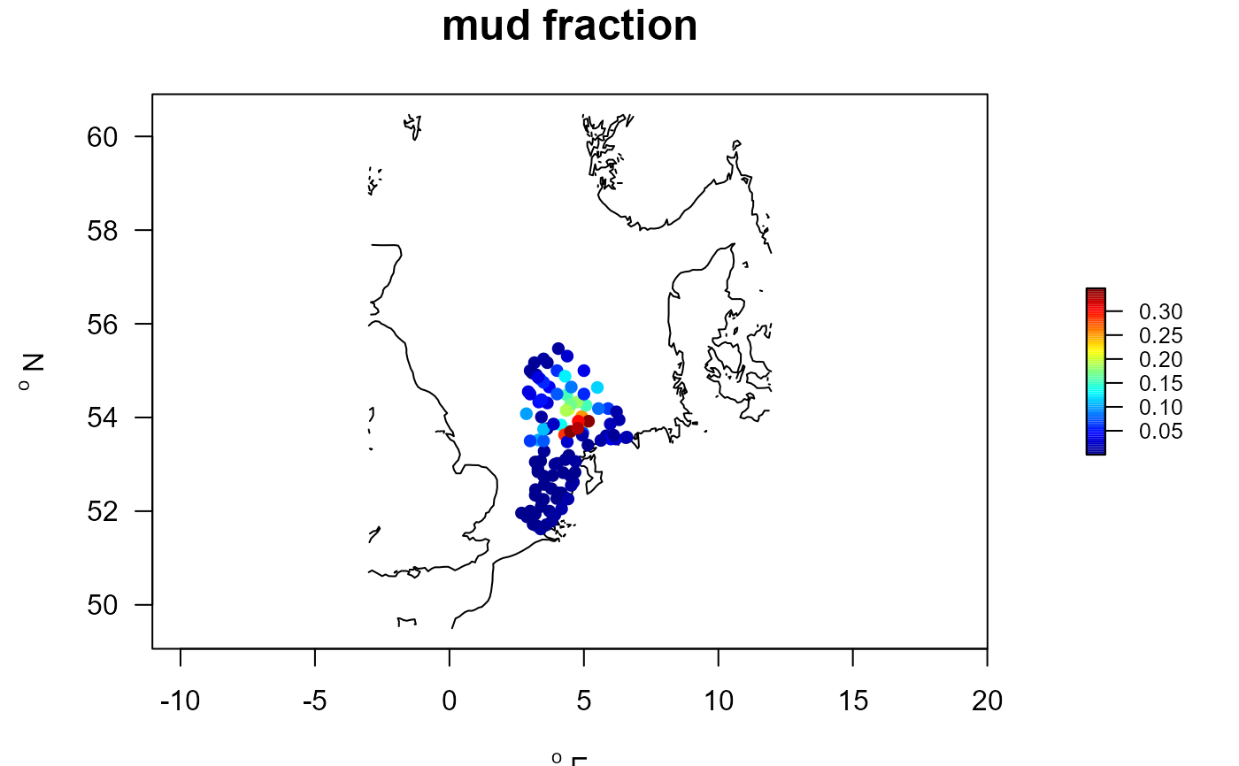
 # mud, plotted on large Northsea map
with(MWTLabiot, map_key(x, y, colvar = mud,
contours = NSBS$contours,
main = "mud fraction",
pch = 16))
# mud, plotted on large Northsea map
with(MWTLabiot, map_key(x, y, colvar = mud,
contours = NSBS$contours,
main = "mud fraction",
pch = 16))
 # show the different abiotic data sets
metadata(MWTL$abiotics)
#> name description units
#> 1 depth water depth m
#> 2 D50 Median grain size micrometer
#> 3 mud mud fraction (<63 um) -
#> 4 sand sand fraction (64 -2000 um) -
#> 5 gravel gravel fraction (>2000 um) -
#> 6 salinity salinity
#> 7 porosity volumetric water content -
#> 8 permeability permeability m2
#> 9 POC particulate organic C in sediment %
#> 10 TN total N in sediment %
#> 11 surfaceCarbon particulate organic C in upper cm %
#> 12 surfaceNitrogen total N in upper cm %
#> 13 orbitalVelMean mean orbital velocity m/s
#> 14 orbitalVelMax maximal orbital velocity m/s
#> 15 tidalVelMean mean tidal velocity m/s
#> 16 tidalVelMax maximal tidal velocity m/s
#> 17 bedstress bed shear stress Pa
#> 18 EUNIScode EUNIScode -
#> 19 DRB swept area ratio for dredge m2/m2/year
#> 20 OT swept area ratio for otter trawl m2/m2/year
#> 21 SN swept area ratio for seines m2/m2/year
#> 22 TBB swept area ratio for beam trawl m2/m2/year
#> 191 sar swept area ratio (fisheries), DRB +OT +SN +TBB m2/m2/year
#> 201 subsar swept area ratio (fisheries) > 2cm m2/m2/year
#> 211 gpd gear penetration depth cm
##-----------------------------------------------------
## COMBINATIONS
##-----------------------------------------------------
NSsp_abi <- merge(MWTL$density, MWTL$sediment)
ECH <- subset(NSsp_abi,
subset = taxon=="Echinocardium")
with(ECH, points2D(D50, density, colvar = density,
log = "xc", pch = 16))
# show the different abiotic data sets
metadata(MWTL$abiotics)
#> name description units
#> 1 depth water depth m
#> 2 D50 Median grain size micrometer
#> 3 mud mud fraction (<63 um) -
#> 4 sand sand fraction (64 -2000 um) -
#> 5 gravel gravel fraction (>2000 um) -
#> 6 salinity salinity
#> 7 porosity volumetric water content -
#> 8 permeability permeability m2
#> 9 POC particulate organic C in sediment %
#> 10 TN total N in sediment %
#> 11 surfaceCarbon particulate organic C in upper cm %
#> 12 surfaceNitrogen total N in upper cm %
#> 13 orbitalVelMean mean orbital velocity m/s
#> 14 orbitalVelMax maximal orbital velocity m/s
#> 15 tidalVelMean mean tidal velocity m/s
#> 16 tidalVelMax maximal tidal velocity m/s
#> 17 bedstress bed shear stress Pa
#> 18 EUNIScode EUNIScode -
#> 19 DRB swept area ratio for dredge m2/m2/year
#> 20 OT swept area ratio for otter trawl m2/m2/year
#> 21 SN swept area ratio for seines m2/m2/year
#> 22 TBB swept area ratio for beam trawl m2/m2/year
#> 191 sar swept area ratio (fisheries), DRB +OT +SN +TBB m2/m2/year
#> 201 subsar swept area ratio (fisheries) > 2cm m2/m2/year
#> 211 gpd gear penetration depth cm
##-----------------------------------------------------
## COMBINATIONS
##-----------------------------------------------------
NSsp_abi <- merge(MWTL$density, MWTL$sediment)
ECH <- subset(NSsp_abi,
subset = taxon=="Echinocardium")
with(ECH, points2D(D50, density, colvar = density,
log = "xc", pch = 16))
 # add station coordinates
ECH <- merge(ECH, MWTL$stations)
##-----------------------------------------------------
## From long format to wide format (stations x species)
##-----------------------------------------------------
NSwide <- with (MWTL$density,
l2w_density(descriptor = station,
taxon = taxon,
value = density,
averageOver = year))
PP <- princomp(t(NSwide[,-1]))
if (FALSE) { # \dontrun{
biplot(PP)
} # }
##-----------------------------------------------------
## Community weighted mean score.
##-----------------------------------------------------
# Traits estimated for absences, by including taxonomy
NStrait.lab <- metadata(Traits_nioz)
trait.cwm <- get_trait_density (wide = NSwide,
trait = Traits_nioz,
taxonomy = Taxonomy,
trait_class = NStrait.lab$trait,
trait_score = NStrait.lab$score,
scalewithvalue = TRUE)
head(trait.cwm, n=c(3,4))
#> descriptor Age.at.maturity Annual.fecundity Biodeposition
#> 1 BREEVTN02 0.3310606 0.3980992 0.2000581
#> 2 BREEVTN03 0.2892671 0.4141280 0.2282032
#> 3 BREEVTN04 0.1056754 0.2908392 0.1369188
Stations.traits <- merge(MWTL$stations, trait.cwm,
by.x = "station", by.y = "descriptor")
##-----------------------------------------------------
## Maps
##-----------------------------------------------------
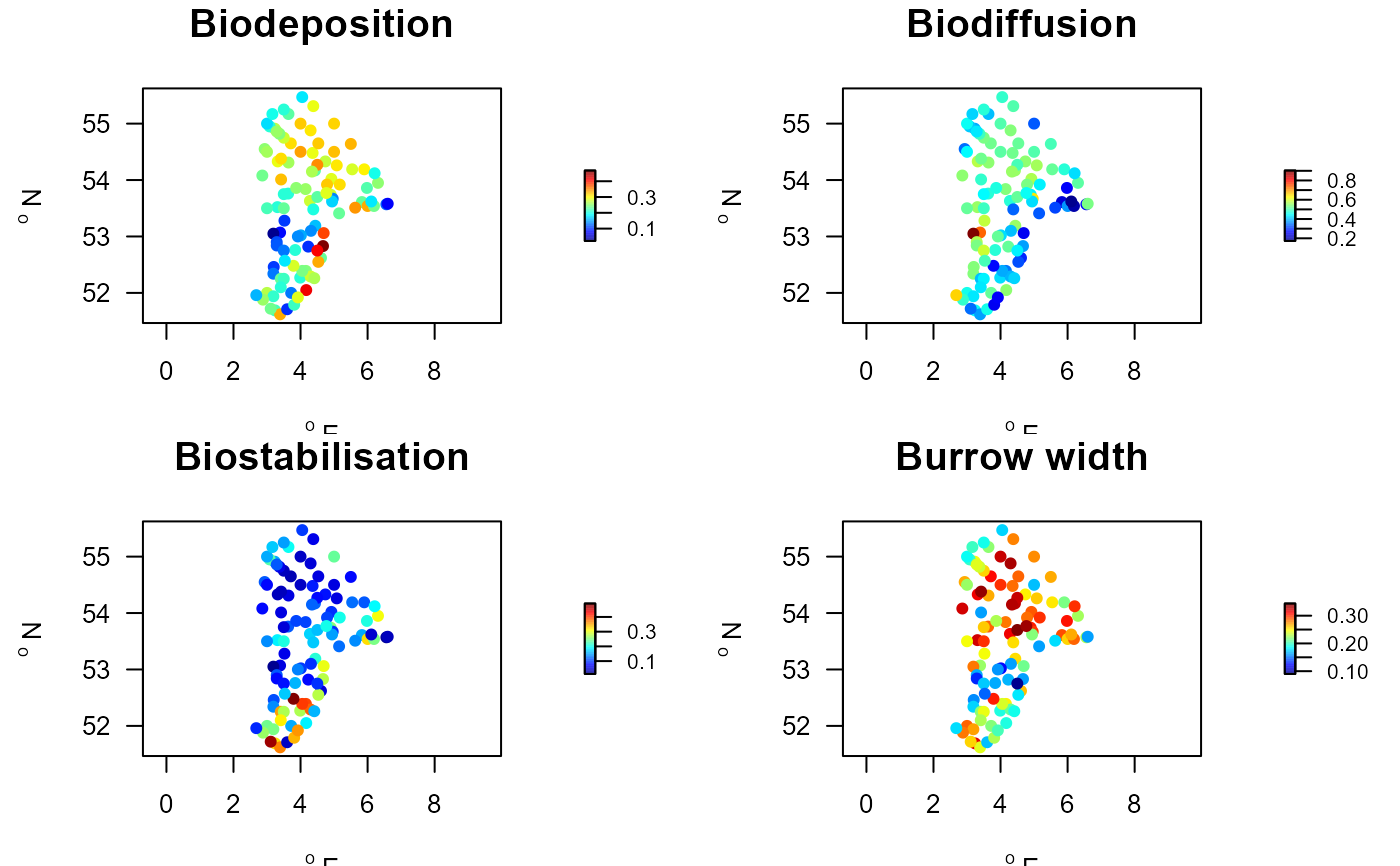
par(mfrow=c(2,2))
with(Stations.traits,
map_key(x, y, colvar = Biodeposition,
main = "Biodeposition",
pch = 16))
#> Warning: no non-missing arguments to min; returning Inf
#> Warning: no non-missing arguments to max; returning -Inf
with(Stations.traits,
map_key(x, y, colvar = Biodiffusion,
main = "Biodiffusion",
pch = 16))
#> Warning: no non-missing arguments to min; returning Inf
#> Warning: no non-missing arguments to max; returning -Inf
with(Stations.traits,
map_key(x, y, colvar = Biostabilisation,
main = "Biostabilisation",
pch = 16))
#> Warning: no non-missing arguments to min; returning Inf
#> Warning: no non-missing arguments to max; returning -Inf
with(Stations.traits,
map_key(x, y, colvar = Burrow.width,
main = "Burrow width",
pch = 16))
#> Warning: no non-missing arguments to min; returning Inf
#> Warning: no non-missing arguments to max; returning -Inf
# add station coordinates
ECH <- merge(ECH, MWTL$stations)
##-----------------------------------------------------
## From long format to wide format (stations x species)
##-----------------------------------------------------
NSwide <- with (MWTL$density,
l2w_density(descriptor = station,
taxon = taxon,
value = density,
averageOver = year))
PP <- princomp(t(NSwide[,-1]))
if (FALSE) { # \dontrun{
biplot(PP)
} # }
##-----------------------------------------------------
## Community weighted mean score.
##-----------------------------------------------------
# Traits estimated for absences, by including taxonomy
NStrait.lab <- metadata(Traits_nioz)
trait.cwm <- get_trait_density (wide = NSwide,
trait = Traits_nioz,
taxonomy = Taxonomy,
trait_class = NStrait.lab$trait,
trait_score = NStrait.lab$score,
scalewithvalue = TRUE)
head(trait.cwm, n=c(3,4))
#> descriptor Age.at.maturity Annual.fecundity Biodeposition
#> 1 BREEVTN02 0.3310606 0.3980992 0.2000581
#> 2 BREEVTN03 0.2892671 0.4141280 0.2282032
#> 3 BREEVTN04 0.1056754 0.2908392 0.1369188
Stations.traits <- merge(MWTL$stations, trait.cwm,
by.x = "station", by.y = "descriptor")
##-----------------------------------------------------
## Maps
##-----------------------------------------------------
par(mfrow=c(2,2))
with(Stations.traits,
map_key(x, y, colvar = Biodeposition,
main = "Biodeposition",
pch = 16))
#> Warning: no non-missing arguments to min; returning Inf
#> Warning: no non-missing arguments to max; returning -Inf
with(Stations.traits,
map_key(x, y, colvar = Biodiffusion,
main = "Biodiffusion",
pch = 16))
#> Warning: no non-missing arguments to min; returning Inf
#> Warning: no non-missing arguments to max; returning -Inf
with(Stations.traits,
map_key(x, y, colvar = Biostabilisation,
main = "Biostabilisation",
pch = 16))
#> Warning: no non-missing arguments to min; returning Inf
#> Warning: no non-missing arguments to max; returning -Inf
with(Stations.traits,
map_key(x, y, colvar = Burrow.width,
main = "Burrow width",
pch = 16))
#> Warning: no non-missing arguments to min; returning Inf
#> Warning: no non-missing arguments to max; returning -Inf
 ##-----------------------------------------------------
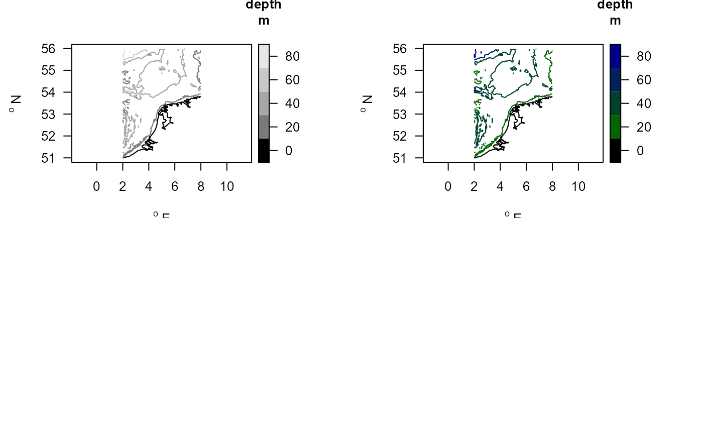
## Show the depth contours
##-----------------------------------------------------
map_key(contours = MWTL$contours, draw.levels = TRUE, key.levels = TRUE)
# Use a different color scheme
collev <- function(n)
c("black", ramp.col(col = c("darkgreen", "darkblue"),
n = n-1))
map_key(contours = MWTL$contours,
draw.levels = TRUE, col.levels = collev,
key.levels = TRUE)
##-----------------------------------------------------
## Fishing data
##-----------------------------------------------------
metadata(MWTL$sar)
#> $data
#> name description units
#> 1 sandy sandy sediment (based on high/low dimensional) or not -
#> 2 year year of the fishing -
#> 3 gear metier; TBB, OT: beam, otter trawl; DRB: dredge, SN: seine -
#> 4 sar annual swept area ratios for the surface (0-2cm) /yr
#> 5 gpd estimated gear penetration depths cm
#>
# Sum fishing per year, per station
MWTLfish <- tapply(X = MWTL$sar$sar,
INDEX = list(MWTL$sar$station, MWTL$sar$year),
FUN = sum)
matplot(x = as.double(colnames(MWTLfish)),
y = t(MWTLfish),
xlab = "year", ylab = "m2/m2/yr",
main = "fishing intensity MWTL stations",
type = "l", log= "y")
##-----------------------------------------------------
## Show the depth contours
##-----------------------------------------------------
map_key(contours = MWTL$contours, draw.levels = TRUE, key.levels = TRUE)
# Use a different color scheme
collev <- function(n)
c("black", ramp.col(col = c("darkgreen", "darkblue"),
n = n-1))
map_key(contours = MWTL$contours,
draw.levels = TRUE, col.levels = collev,
key.levels = TRUE)
##-----------------------------------------------------
## Fishing data
##-----------------------------------------------------
metadata(MWTL$sar)
#> $data
#> name description units
#> 1 sandy sandy sediment (based on high/low dimensional) or not -
#> 2 year year of the fishing -
#> 3 gear metier; TBB, OT: beam, otter trawl; DRB: dredge, SN: seine -
#> 4 sar annual swept area ratios for the surface (0-2cm) /yr
#> 5 gpd estimated gear penetration depths cm
#>
# Sum fishing per year, per station
MWTLfish <- tapply(X = MWTL$sar$sar,
INDEX = list(MWTL$sar$station, MWTL$sar$year),
FUN = sum)
matplot(x = as.double(colnames(MWTLfish)),
y = t(MWTLfish),
xlab = "year", ylab = "m2/m2/yr",
main = "fishing intensity MWTL stations",
type = "l", log= "y")