Benthic density and trait databases in R-package Btrait

Introduction.

The R-package Btrait facilitates working with a combination of biological density, trait, and taxonomic data. It contains:

functions for working with density and trait data (getDensity, getTraits, getTraitDensity, …),
two data sets with macrobenthos species density and biomass data from the Northsea (MWTL, NSBS),
data sets with functional trait data (Traits_nioz, Traits_cefas, Traits_Db, Traits_irr).

The main vignette Btrait demonstrates how to use the functions in the package using a small data set.

This vignette introduces the benthic databases.

The Northsea macrobenthos density data

The macrobenthos are animals living in the sediment and that are retained on a sieve with mesh size of 1mm. They are important for the ecosystem services they deliver, i.e. by their impact on biogeochemistry (nutrient dynamics), and as they are an important food source to fishes.

Btrait contains two data sets that contain Northsea macrobenthos density and biomass:

the MWTL data, (one or three-) yearly data from the Dutch part of the North Sea, and
the NSBS (Northsea Benthos Survey) data, a one-time survey that covers the entire North Sea.

The MWTL dataset

The Dutch Rijkswaterstaat (RWS) has performed regular macrobenthos sampling in the Dutch part of the Northsea, from 1995 till 2018. This activity is called “MWTL monitoring” .

The monitoring was done on a yearly basis from 1995 till 2010, after which sampling was less frequent, occurring in 2012, 2015, 2018. Not all stations were always sampled though; 5 stations were sampled 18 rather than 19 times; another 6 stations were sampled less or equal than 12 times.

The sampling region extends inbetween (2.68, 6.6) dg East and (51.62, 55.47) dg North, with water depths varying in between (5.8, 53.7) m.

There are 41849 records in this macrofauna data set for 103 stations.

Sampling started in 01-03-2001; the last sample taken in 31-05-1995.

Taxonomy was adjusted to account for rare taxa, determined on a high taxonomic level.

The sampled organisms belonged to 400 different taxa (after adjustment); before adjustment 525 taxa were distinguished.

Biomass, expressed in ash-free dry weight per square m ([gDWT/m2]), was estimated at similar taxonomic level as density estimates.

The data from these monitoring campaigns are available from RWS; they have been and made available in the framework of the EMODNET biology project.

Note that this database is atypical in the sense that sometimes the station x sampling date x taxon can be present multiple times. This is because sometimes organisms of the same taxon but very different sizes were weighed separately, or because taxa were later reclassified to another taxon that was already available. One example of such double occurrence is:

DOUBLE <- subset(MWTL$density, 
   subset=(station=="TERHDE1" & year==2018 & taxon == "Donax vittatus"))

knitr::kable(DOUBLE, caption = "example of a double occurrence in the MWTL dataset",
             row.names=FALSE)

example of a double occurrence in the MWTL dataset
station	date	year	taxon	density	biomass	taxon.original
TERHDE1	16-03-2018	2018	Donax vittatus	38.46154	1.2884615	Donax vittatus
TERHDE1	16-03-2018	2018	Donax vittatus	38.46154	0.0064103	Donax vittatus

The NSBS dataset

In 1986, a large macrofauna survey took place covering the entire Northsea (Heip et al., 1992). Benthic samples were taken in a standardised way, on a regular grid covering the whole of the North Sea, and analysed by scientists from 10 laboratories. Extensive work was done to standardise taxonomy and identifications across the different laboratories.

The sampling region for these data extends inbetween (-3, 9) dg East and (51, 60.75) dg North, depths varying inbetween (4.1999998, 195.1999969) m.

There are 11150 records in this macrofauna data set for 234 stations.

Sampling took place in 1986; the actual sampling time was not recorded.

The sampled organisms belonged to 552 different taxa.

Biomass, expressed in ash-free dry weight per square m ([gDWT/m2]), was estimated at low taxonomic level, distinguishing between Polychaeta (class), Mollusca, Echinodermata, Crustacea (phylum) or even at higher level (Animalia). As this is at much lower resulution as density estimates, biomass is stored in a separate data.frame.

Structure of the density data sets

The density data have been gathered in a list called MWTL and NSBS that contains a number of data.frames:

MWTL$density, NSBS$density, NSBS$biomass: the species (taxon) density and biomass data, in long format. The MWTL$density data.frame, provides stations, date, taxon, density (ind/m2) and biomass (ashfree dry weight/m2). The column “taxon.original” refers to the original taxon, and “taxon” the selected taxon after ‘taxonomic adjustment’ (see help file, help(“MWTL$density”), for how taxa were adjusted). Density and biomass data are in separate dataframes for the NSBS data.
MWTL$stations, NSBS$stations: coordinates of the stations referred to in MWTL$density and NSBS$density, in WGS84 format.
MWTL$sediment, MWTL$abiotics, MWTL$types, NSBS$abiotics: abiotic conditions from various sources (Wilson et al., 2018; MWTL, Deltares).
MWTL$contours: bathymetric contour lines for quick plotting of the data. Contours were generated by applying the contourLines function from base R (R core team 2021), and are based on high-resolution GEBCO bathymetry data from the Northsea.

The taxonomic relationships between taxa is in a data.frame called Taxonomy, as generated with the worms package (Holstein, 2018).

The positions and names of the MWTL and NSBS stations is in the following figures, where the colors either denote the area (MWTL) or water depths (NSBS).

Each of these data.frames, has a description in its attributes, which can be extracted with the function metadata.

metadata(MWTL$density)

##             name                                description          units
## 1        station                               station name               
## 2           date                    sampling date, a string               
## 3          taxon taxon name, checked by worms, and adjusted               
## 4        density                      species total density individuals/m2
## 5        biomass          species total ash-free dry weight       gAFDW/m2
## 6 taxon.original                        original taxon name

Station positions

We use function mapBtrait to generate figures with station positions, passing the respective contours for each dataset. The R-function merge is used to augment the data.frame types (that contains the area to which each station belongs), with the longitudes (x) and latitudes (y) in the stations data.frame.

MWTLab   <- merge(MWTL$stations, 
                  MWTL$types, by="station")

MWTLab$area <- factor(MWTLab$area)

par(las=1, oma=c(0,0,1,0), cex.axis=1.2, cex.main=2, cex.lab=1.2)
with(MWTLab, 
  mapBtrait(contours=MWTL$contours, x=x, y=y, col=c(1:4)[area], 
            pch=c(15:18)[area], cex=2, main="MWTL station positions", 
            clab="m", draw.levels=TRUE))
with(MWTL$stations, text(x, y+0.05, label=station, cex=0.8, adj=0))
legend ("bottomright", legend=levels(MWTLab$area), col=1:4, pch=15:18, cex=2)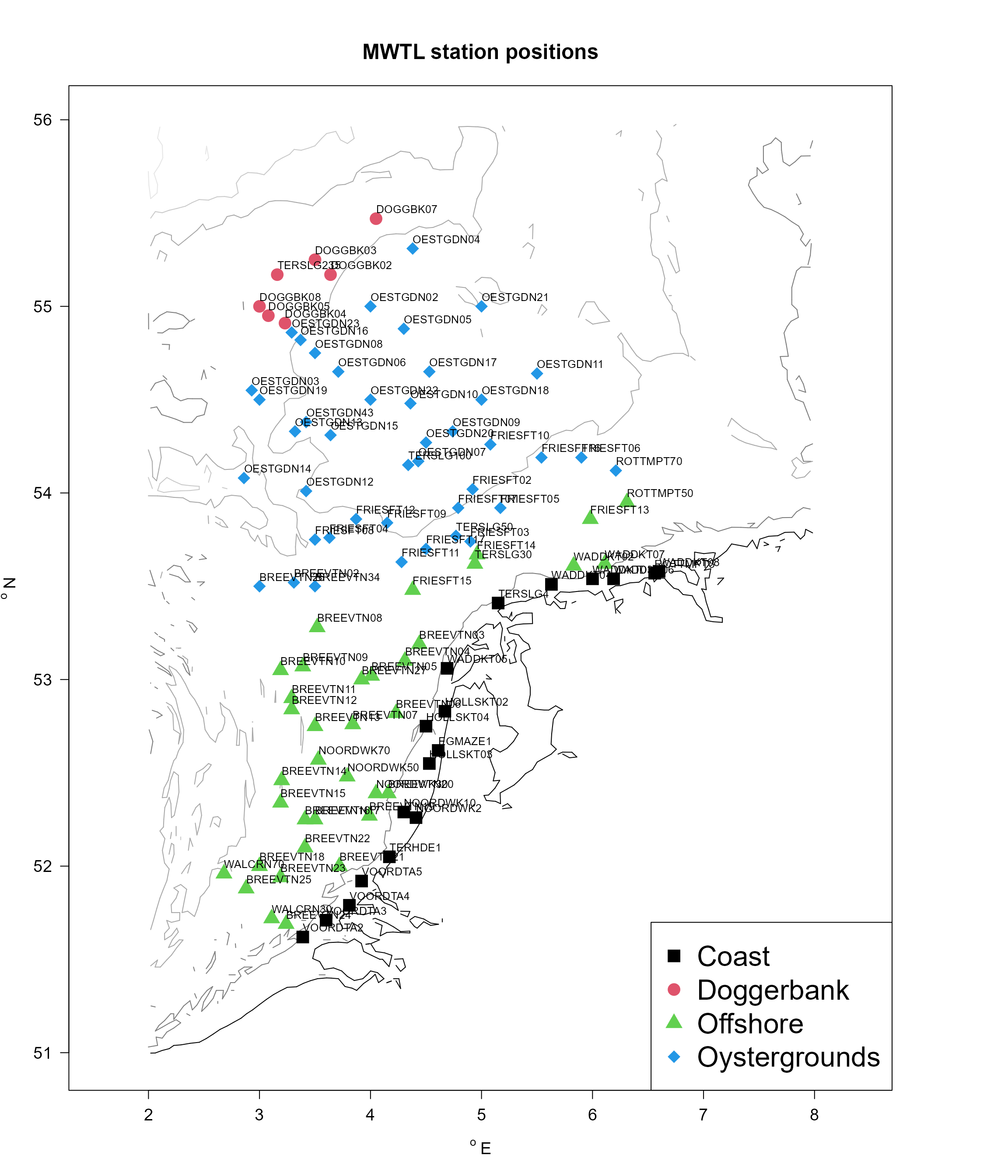

NSBSabio <- merge(NSBS$stations, NSBS$abiotics, by="station")

par(las=1, oma=c(0,0,1,0), cex.axis=1.2, cex.main=2, cex.lab=1.2)
with(NSBSabio, 
  mapBtrait(contours=NSBS$contours, x=x, y=y, colvar=depth, 
            pch=16, cex=2, main="NSBS station positions", 
            clab="m", draw.levels=TRUE))
# remove the "ICES" from the station names
with(NSBS$stations, text(x=x+0.05, y=y+0.08, 
     label=substr(station, 5, 7), cex=0.9, adj=0))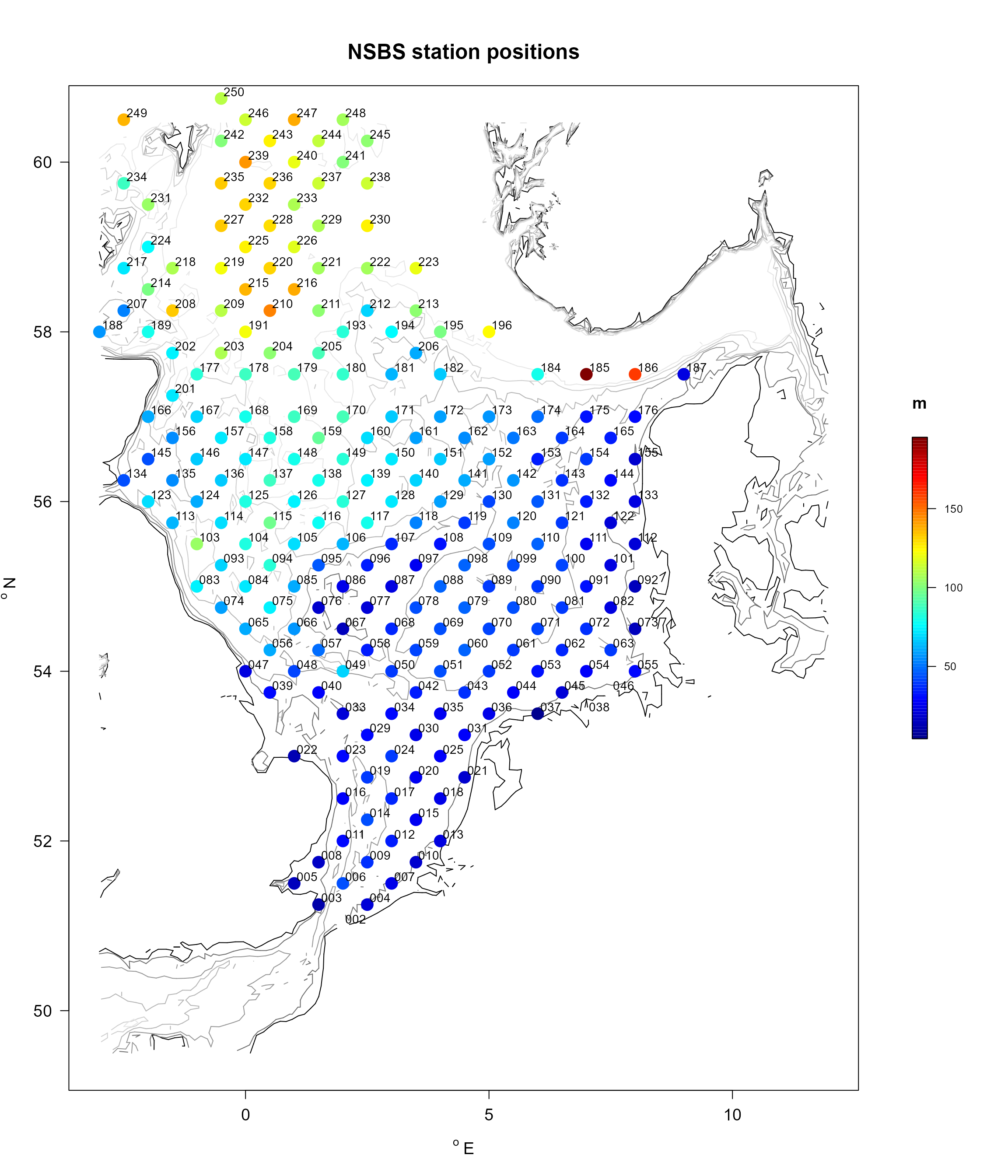

Consistency of the density databases

We test the consistency of both data sets, by looking at the total density, biomass, and number of taxa of stations that were sampled in common.

To find the common stations, we merge the station information of both datasets, by the coordinates (x, y):

Common <- merge(MWTL$stations, 
                NSBS$stations, 
                by=c("x", "y"))
colnames(Common)[3:4] <- c("MWTL", "NSBS")
knitr::kable(Common, caption="stations in common by MWTL and NSBS dataset",
             row.names=FALSE)

stations in common by MWTL and NSBS dataset
x	y	MWTL	NSBS
3.0	52.00	BREEVTN18	ICES012
3.0	53.50	BREEVTN26	ICES034
3.0	54.50	OESTGDN19	ICES068
3.0	55.00	DOGGBK08	ICES087
3.5	52.25	BREEVTN17	ICES015
3.5	52.75	BREEVTN13	ICES020
3.5	53.75	FRIESFT08	ICES042
3.5	54.75	OESTGDN08	ICES078
3.5	55.25	DOGGBK03	ICES097
4.0	54.50	OESTGDN22	ICES069
4.0	55.00	OESTGDN02	ICES088
4.5	52.75	HOLLSKT04	ICES021
5.0	54.50	OESTGDN18	ICES070
5.0	55.00	OESTGDN21	ICES089

To test whether the density, biomass and number of taxa are comparable in both datasets, we estimate these quantities for the common stations and plot them versus one another, adding the 1:1 line.

The biomass and density data are compatible. The total number of taxa found in the NSBS data set is much lower than in the MWTL data set, but this is not surprising, as the MWTL data were sampled on a regular basis over 19 years, whereas the NSBS data were gathered in a one-time event.

In the figures below, maps of total density and number of taxa are created for both data sets.

MWTL.summ <-  with (MWTL$density, 
    getSummary(descriptor  = station, 
               averageOver = year, 
               taxon       = taxon, 
               value       = density))

NSBS.summ <-  with (NSBS$density, 
    getSummary(descriptor = station, 
               taxon      = taxon, 
               value      = density))

par(mfrow=c(2,2))
par(las=1, oma=c(1,1,1,1), cex.main=2)

with(merge(MWTL$stations, MWTL.summ$density, by=1), 
  mapBtrait(contours=MWTL$contours, x=x, y=y, colvar=density, 
            pch=18, cex=2, main="MWTL total density",  
            clab="ind/m2", draw.levels=TRUE))
with(merge(NSBS$stations, NSBS.summ$density, by=1), 
  mapBtrait(contours=NSBS$contours, x=x, y=y, colvar=density, 
            pch=18, cex=2, main="NSBS total density", 
            clab="ind/m2", draw.levels=TRUE))

with(merge(MWTL$stations, MWTL.summ$taxa, by=1), 
  mapBtrait(contours=MWTL$contours, x=x, y=y, colvar=taxa, 
            pch=18, cex=2, main="MWTL number of taxa", 
            clab="/m2", draw.levels=TRUE))
with(merge(NSBS$stations, NSBS.summ$taxa, by=1), 
  mapBtrait(contours=NSBS$contours, x=x, y=y, colvar=taxa, 
            pch=18, cex=2, main="NSBS number of taxa", 
            clab="/m2", draw.levels=TRUE))

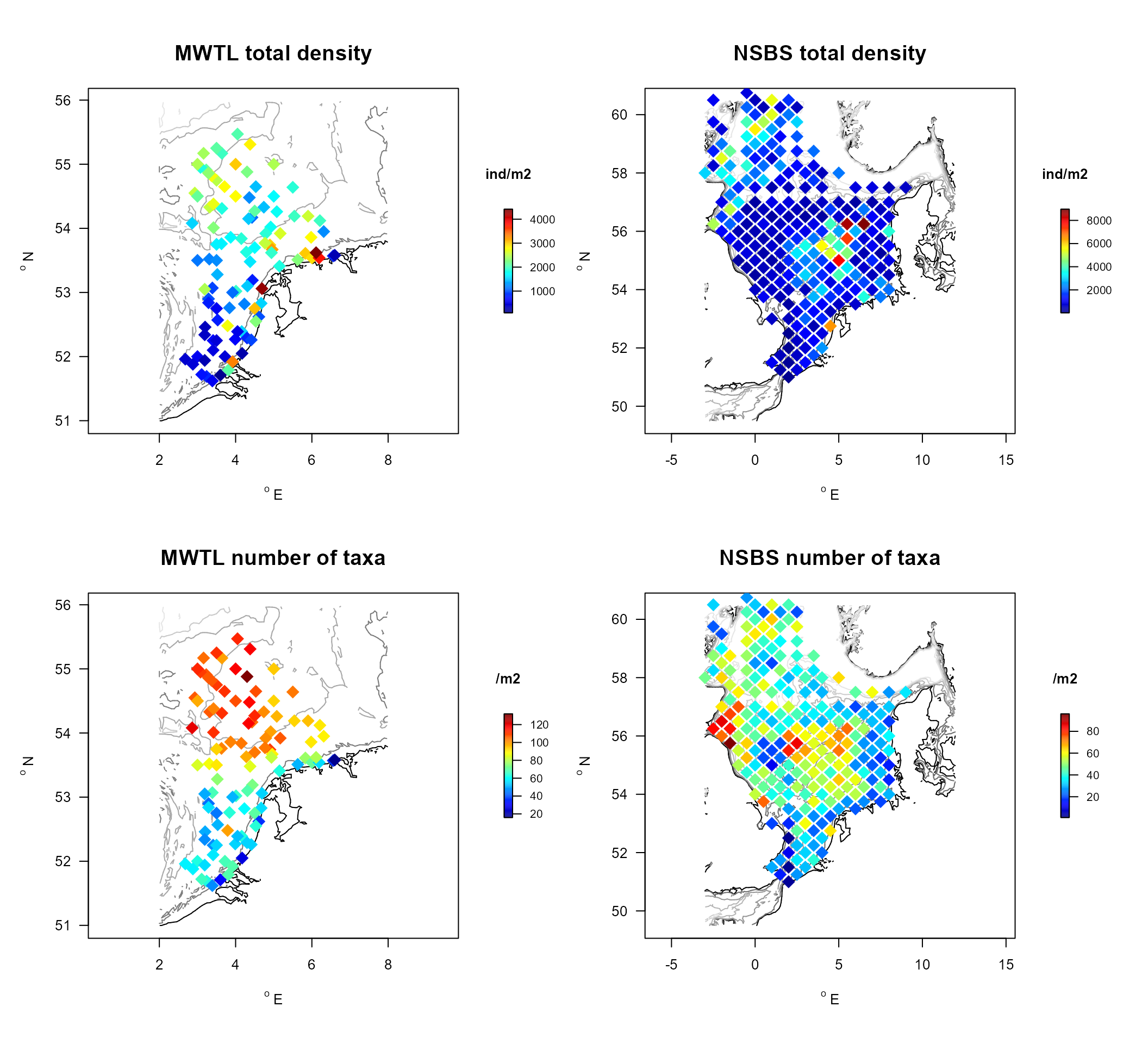
Benthic trait databases

Four benthic trait datasets are included in R-package Btrait:

Beauchard et al. (2021, in press) compiled 32 traits from 281 taxa. The traits comprise both “functional effects” traits, which affect ecosystem properties, and “response” traits, which affect a species’ response from changes in the environment, such as disturbance. The traits are fuzzy coded; taxonomic level is mainly on species level. This extensive trait database is called Traits_nioz.
Clare et al (2022) compiled 10 traits from 1025 taxa; mainly on genus level. These fuzzy coded traits are in Traits_cefas.
Traits necessary to estimate the Bioturbation potential of 1060 taxa were compiled by Queiros et al 2013; these data were extended by data from ilvo (courtesy Gert van Hoey). The traits in this data set are numerical traits, i.e. a value is assigned to the reworking (Ri), mobility (Mi) and feeding type (Fti) traits. Many traits are recorded at species level. These traits are in Traits_Db.
Traits necessary to estimate the Bio-irrigation potential (as in Wrede et al., 2018) were derived from the nioz trait database; it contains numeric values for bottom traits (BT), for injection depth (ID), and for feeding type (FT), for 281 taxa. The traits in this data set are numerical traits, i.e. a value is assigned to them. These traits are in Traits_Irr.

Species groups

The data.frame Groups contains 11 typological species groups representing sea floor functions, as derived from a cluster analysis on species traits by Beauchard et al. (in press).

Structure of the trait databases

The trait information is stored in a ($taxa \times traits$) data.frame, where the first column represents the taxon name, and subsequent columns have the trait scores for the various trait modalities; the column names represent the trait modalities.

For example, the first part of the NIOZ trait data is:

head(Traits_nioz, n=c(3,3))

##                   taxon ET1.M1 ET1.M2
## 1          Abludomelita    0.5    0.5
## 2 Abludomelita obtusata    0.5    0.5
## 3             Abra alba    0.0    0.5

where ET1.M1 is shorthand for modality 1 of the effect trait 1.

For each trait database, the meaning of the traits and the modalities is explained in the attribute description of the data.frame, which can be extracted with the function metadata. Below are the first two rows from the description in the Traits_nioz:

head(metadata(Traits_nioz), n=2)

##   colname                         trait modality indic value score units
## 1  ET1.M1 Substratum depth distribution        0     1   0.0  1.00    cm
## 2  ET1.M2 Substratum depth distribution      0-5     1   2.5  0.75    cm

The description attribute is a data.frame with the following columns: colname, trait, modality, indic, value, score and units.

Here

Finding traits for macrofauna taxa is a lot of work, and many of the taxa that are recorded in the benthos databases are not represented in the trait databases.

With respect to the northsea data sets (MWTL and NSBS) for instance, the percentage of taxa not represented in the trait databases is:

MWTL	NSBS
47.75	63.04348
85.25	90.94203
24.75	25.90580

Note that the low presence of the species in the cefas Trait dataset is due to the fact that this dataset has the traits recorded on genus level, while the MWTL and NSBS datasets provide data mainly at species level.

Taxonomy

A taxonomic tree that comprises the taxonomic information for all taxa in the trait databases and in the density databases is included in database Taxonomy.

The names of the taxa in all databases has been checked with the worms database, using R-package worms (Holstein, 2018).

Consistency of the trait databases

A number of traits are present in both the cefas and nioz datasets; they are

Body Length (nioz) and Maximum size (cefas).
Life span (nioz) and Lifespan (cefas).
Substratum depth distribution (nioz) and Sediment position (cefas).

Both trait datasets also record the feeding type/feeding modes.

These data are represented by:

cefas_select <- subset(metadata(Traits_cefas), 
     trait %in% c("Maximum size", "Lifespan", "Sediment position"))
nioz_select <- subset(metadata(Traits_nioz), 
     trait %in% c("Body length", "Life span", "Substratum depth distribution"))

knitr::kable(cefas_select[,c(1,2,3,5,7)], caption="CEFAS traits in common",
             row.names=FALSE)

CEFAS traits in common
colname	trait	modality	value	units
sr_Less_than_10	Maximum size	<10	5.0	mm
sr_11_to_20	Maximum size	11-20	15.0	mm
sr_21_to_100	Maximum size	21-100	60.0	mm
sr_101_to_200	Maximum size	101-200	150.0	mm
sr_201_to_500	Maximum size	201-500	350.0	mm
sr_More_than_500	Maximum size	>500	750.0	mm
l_Less_than_1	Lifespan	<1	0.5	years
l_1_to_3	Lifespan	1-3	2.0	years
l_3_to_10	Lifespan	3-10	6.5	years
l_More_than_10	Lifespan	>10	15.0	years
sp_Surface	Sediment position	Surface	0.0	cm
sp_Shallow_infauna_0_to_5cm	Sediment position	Shallow_infauna_0_to_5cm	2.5	cm
sp_Mid_depth_infauna_5_to_10cm	Sediment position	Mid_depth_infauna_5_to_10cm	7.5	cm
sp_Deep_infauna_more_than_10cm	Sediment position	Deep_infauna_more_than_10cm	15.0	cm

knitr::kable(nioz_select [,c(1,2,3,5,7)], caption="NIOZ traits in common",
             row.names=FALSE)

NIOZ traits in common
colname	trait	modality	value	units
ET1.M1	Substratum depth distribution	0	0.0	cm
ET1.M2	Substratum depth distribution	0-5	2.5	cm
ET1.M3	Substratum depth distribution	5-15	10.0	cm
ET1.M4	Substratum depth distribution	15-30	22.5	cm
ET1.M5	Substratum depth distribution	>30	30.0	cm
RT2.M1	Body length	<1	0.5	mm
RT2.M2	Body length	1-3	2.0	mm
RT2.M3	Body length	3-10	6.5	mm
RT2.M4	Body length	10-20	15.0	mm
RT2.M5	Body length	20-50	35.0	mm
RT7.M1	Life span	<1	0.5	year
RT7.M2	Life span	1-3	2.0	year
RT7.M3	Life span	3-10	6.5	year
RT7.M4	Life span	10-20	15.0	year
RT7.M5	Life span	>20	30.0	year

The traits in the cefas database are now matched with those in the nioz database, with function getTrait. The species data in the nioz database are calculated on genus level, so that they can be compared with the cefas data. This is done by passing the taxonomic tree up to genus level. For a large number of genera in the cefas database, the traits could not be found; they are removed (they are NA in the returned data).

# Select nioz traits for the taxa in the cefas database
TR_nioz <- getTrait(
  taxon    = Traits_cefas$taxon,   
  trait    = Traits_nioz[,c("taxon", nioz_select$colname)],
  taxonomy = Taxonomy[,c("taxon", "genus")]
  )
TR_nioz <- na.omit(TR_nioz)
TR_nioz <- TR_nioz[order(TR_nioz$taxon),]

Of the 1025 taxa in the cefas data set, the traits of only 193 taxa could be calculated from the nioz data.

The data are converted to crisp format, and merged with the crisp cefas data.

trnioz <- fuzzy2crisp(
  trait       = TR_nioz,
  trait.class = nioz_select$trait,
  trait.score = nioz_select$value
)
trcefas <- fuzzy2crisp(  
  trait       = Traits_cefas[,c("taxon", cefas_select$colname)],
  trait.class = cefas_select$trait,
  trait.score = cefas_select$value
)
trall <- merge(trnioz, trcefas, by=1)
dim(trall)

## [1] 193   7

trall[1:2,]

##          taxon Body.length Life.span Substratum.depth.distribution Lifespan
## 1 Abludomelita         0.5       0.5                        1.2500      0.5
## 2         Abra         2.0       2.0                        3.4375      2.0
##   Maximum.size Sediment.position
## 1            5               0.0
## 2           15               2.5

The feeding type in the nioz data and the feeding mode from cefas are extracted and made consistent.

CEFAS feeding types
colname	trait	modality	indic	value	score	units	description
f_Suspension	Feeding mode	Suspension	9	0.0	0.0	-	Feeds on particulate food resources suspended in the water column.
f_Surface_deposit	Feeding mode	Surface_deposit	9	0.2	0.2	-	Feeds on detritus (including algal material) on the sediment surface.
f_Subsurface_deposit	Feeding mode	Subsurface_deposit	9	0.4	0.4	-	Feeds on detritus located within the sediment matrix.
f_Scavenger	Feeding mode	Scavenger	9	0.6	0.6	-	Feeds on dead animals (carrion).
f_Predator	Feeding mode	Predator	9	0.8	0.8	-	Actively predates on animals (including small zooplankton).
f_Parasite	Feeding mode	Parasite	9	1.0	1.0	-	Derives nutrition from its host organism.

NIOZ feeding types
colname	trait	modality	indic	value	score	units
RT6.M1	Feeding type	Deposit feeder	6	0.0000000	0.0000000	-
RT6.M2	Feeding type	Suspension feeder	6	0.3333333	0.3333333	-
RT6.M3	Feeding type	Herbivore/Grazer	6	0.6666667	0.6666667	-
RT6.M4	Feeding type	Carnivore/Scavenger	6	1.0000000	1.0000000	-

The consistency of the trait databases is shown by plotting the deviation between both datasets. These deviations are very close to 0, showing that both datasets are comparable.

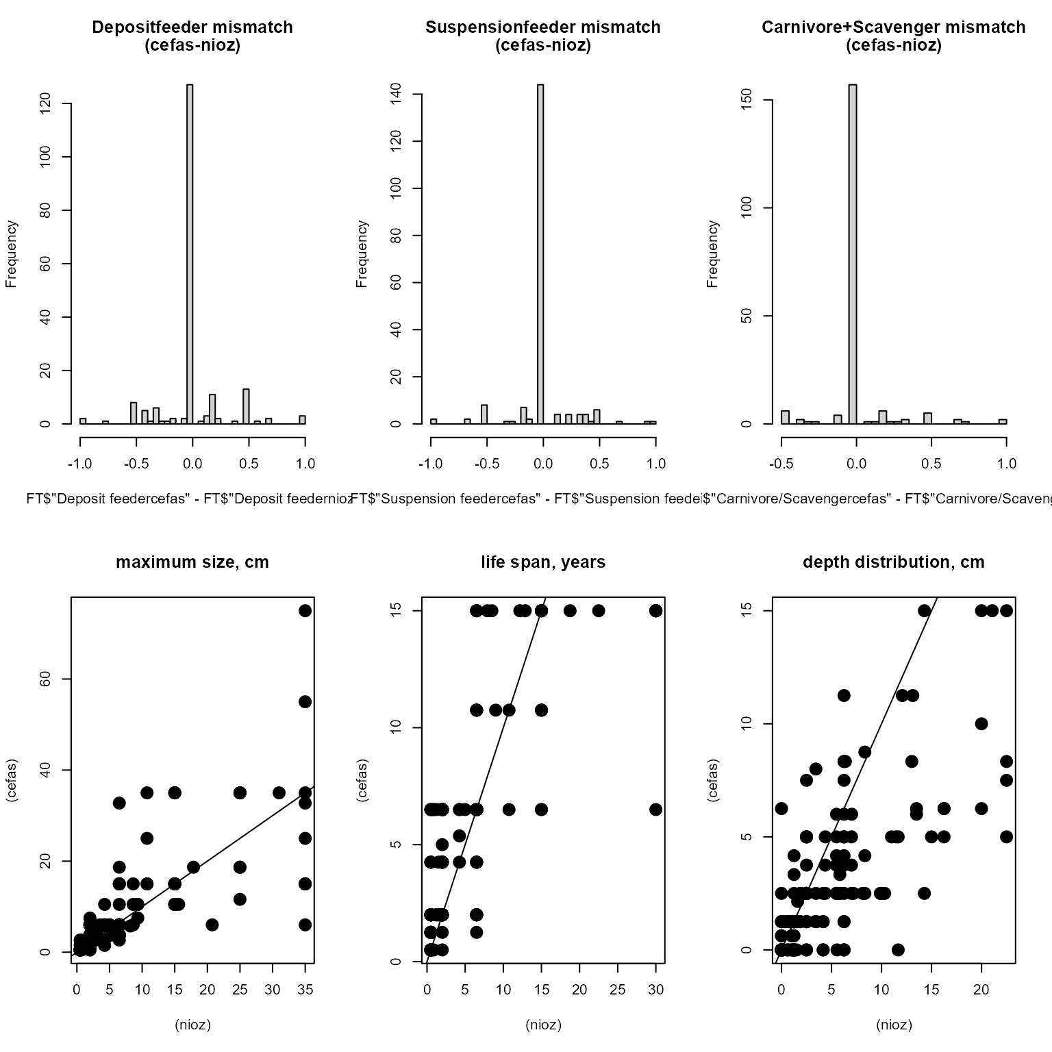
Comparison of common traits in the nioz and cefas database

statistics of deviations between cefas and nioz trait data
Min.	1st Qu.	Mean	3rd Qu.	Max.
-1.00	0.00	0.0130438	0.0	1.0
-1.00	0.00	0.0061662	0.0	1.0
-0.50	0.00	0.0214800	0.0	1.0
-40.00	-1.75	-0.7519293	0.5	29.0
-8.50	-1.50	-0.2101715	0.0	23.5
-6.25	0.00	1.6675702	2.5	17.5

Combining density and trait data

Community Weighted Mean (CWM) of MWTL Northsea data based on cefas traits.

The Community Weighted Mean (CWM) of traits is estimated, based on the (stations x taxon density) and (taxon x traits) matrix; we use the cefas data. In the function getTraitDensity, we pass the value of the modalities (trait.score) of the trait classes, so that the average modality value will be calculated. We also pass the taxonomy table, so that the traits for unknown taxa will be generated, based on their taxonomic relationship.

Tcefas.lab <- metadata(Traits_cefas)

MWTL.cwm <- getTraitDensity(
                descriptor  = MWTL$density$station, 
                taxon       = MWTL$density$taxon, 
                averageOver = MWTL$density$year,
                value       = MWTL$density$density, 

                trait       = Traits_cefas, 
                trait.class = Tcefas.lab$trait, 
                trait.score = Tcefas.lab$value, 
                taxonomy    = Taxonomy)

The mean trait values per station are plotted for the sediment position, the maximum size and the lifespan.

Station.traits <- merge(MWTL$stations, MWTL.cwm, by=1)

par(mfrow=c(1,2), mar=c(3,3,3,2), oma=c(2,2,0,0))
units          <-  rbind(unique(Tcefas.lab[,c("trait", "units")]))
units$colnames <- make.names(units$trait)

ii <- which(units$trait %in% c("Sediment position", "Lifespan"))
for (i in ii)
 mapBtrait(x=Station.traits$x, y=Station.traits$y, contours=MWTL$contours,
      colvar= Station.traits[,units$colnames[i]], 
      cex=2, clab=units[i,2], main=units[i,1], pch=18)

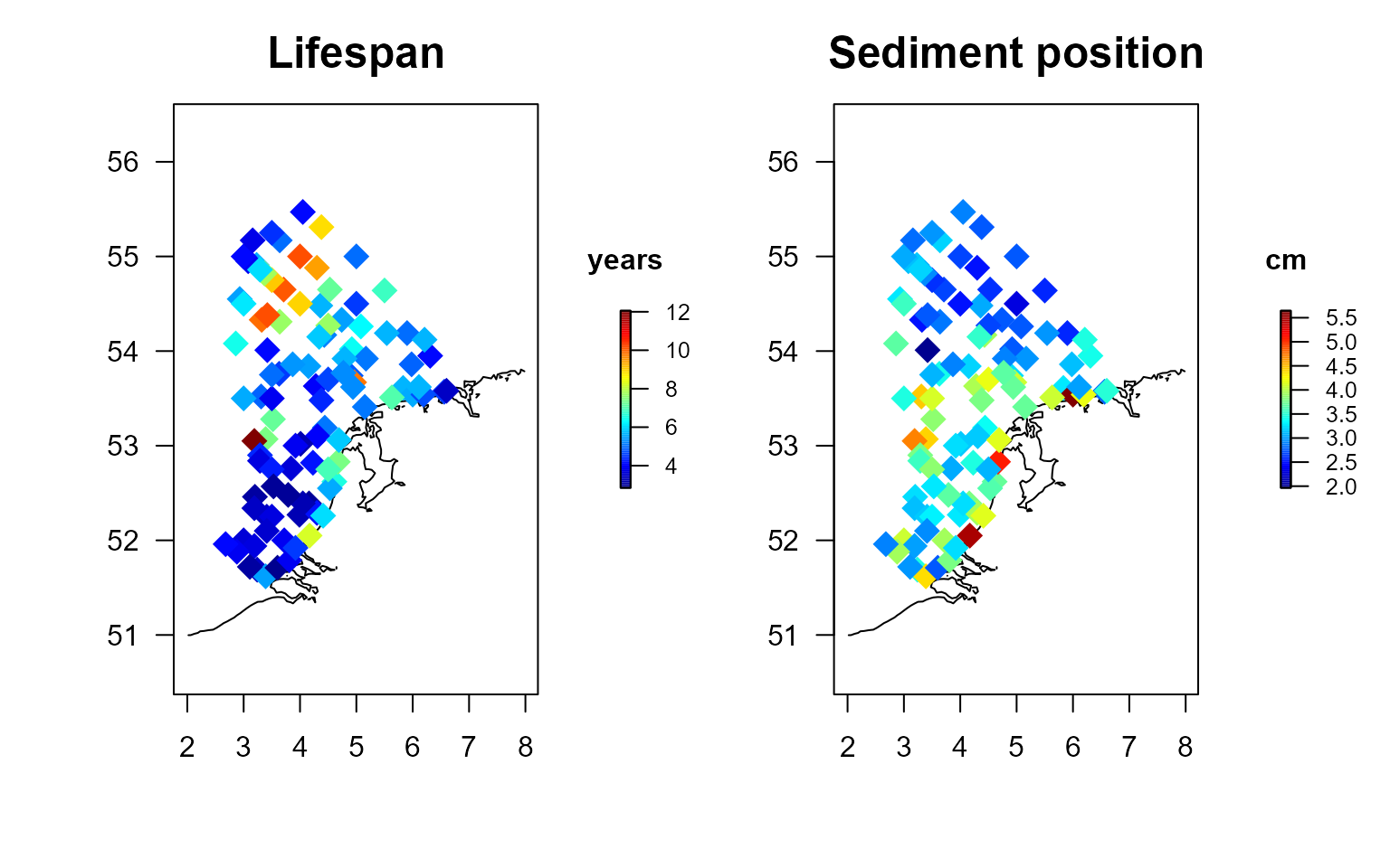
Community weighed trait values based on the MWTL density and cefas trait data

Estimating the bioturbation and bio-irrigation potential

We use the data from the Dutch part of the Northsea, in 1995, to estimate the bioturbation potential index sensu Solan et al., 2004 and Queiros et al., 2013.

The contribution of a species, $i$ to the bioturbation potential ($BPc$) is based on its mean individual weight ($W_i$), the abundance ($A_i$), and its mobility ($M_i$) and sediment reworking mode ($R_i$); the station BPc is then simply the sum of the species bioturbation potential.

\[BPc = \sum_i \sqrt{W_i} \times A_i \times M_i \times R_i\]

Mobility scales, $M_i$ have a value of $1$ for organisms living in a fixed tube, $2$ indicates limited movement; $3$ indicates slow, free movement through the sediment matrix; $4$ indicates free movement, via burrow system.
sediment reworking ($R_i$) takes on the value $1$ for epifauna that bioturbate at the sediment–water interface, $2$ for surficial modifiers; $3$ for upward and downward conveyors; $4$ for biodiffusors; and $5$ for regenerators that excavate holes, transferring sediment at depth to the surface.

The contribution of a species, $i$ to the bio-irrigation potential ($IPc$) (sensu Wrede et al., 2018.), is based on its mean individual weight ($W_i$), the abundance ($A_i$), the burrow type ($BT_i$), feeding TYPE ($FT_i$) and the depth of the injection pocket, in centimeter ($ID_i$); the station $IPc$ is then simply the sum of the species bio-irrigation potential.

\[IPc = \sum_i {W_i}^{3/4} \times A_i \times BT_i \times FT_i \times ID_i\]

Scores for the burrowtype, $BT_i$ are $1$ for epifauna, and species with internal irrigation (e.g. using siphons), $2$ for open irrigation (e.g. U- or Y- shaped burrows), and $3$ for blind ended irrigation (e.g. blind ended burrows, no burrow systems).
Scores for feeding types, $FT_i$ are $1$ for surface filter feeders, $2$ for predators, $3$ for deposit feeders and $4$ for sub surface filter feeders.
Injection pockets, $IP_i$, at depths of 0-2, 2-5, 5-10 and >10 cm depth get an ID score of $1$, $2$, $3$ and $4$ respectively.

The bioturbation index can easily be estimated from the function getDbIndex, and the database Traits_Db. The bioirrigation index can be estimated from the function getIrrIndex, and the database Traits_Irr.

As not all MWTL taxa are represented in Traits_Db or Traits_irr, we use information on closely related species at the nearest taxonomic level, to also provide values for those taxa that are not represented. It suffices to pass the taxonomic information to function getDbIndex or getIrrIndex to achieve this.

The functions return the total bioturbation or bioirrigation index for all stations, and the average BPc or IPC for all taxa.

In the code below, first the Northsea data are selected; we select the data for 1995 only. Then the bioturbation and bioirrigation index are estimated based on these data.

MWTL1995 <- with (MWTL$density, 
     getDensity(descriptor = list(station=station),
                subset     = (year == 1995),
                taxon      = taxon,
                value      = data.frame(density, biomass))) 

MWTLDb <- with(MWTL1995, 
  getDbIndex (descriptor = station, 
              taxon      = taxon, 
              density    = density, 
              biomass    = biomass, 
              trait      = Traits_Db, 
              taxonomy   = Taxonomy))

MWTLIrr <- with(MWTL1995, 
  getIrrIndex(descriptor = station, 
              taxon      = taxon, 
              density    = density, 
              biomass    = biomass, 
              trait      = Traits_irr, 
              taxonomy   = Taxonomy))

Both functions return a list with several data.frames:

descriptor gives the total BPc or IPc value for the descriptor here stations.
taxon gives the average BPc or IPc value for the taxa

MWTLbpc            <- MWTLDb$descriptor
row.names(MWTLbpc) <- NULL
knitr::kable(head(MWTLbpc[order(MWTLbpc$BPc, decreasing=TRUE),], n=10),
             caption="10 stations with largest bioturbation potential",
             row.names=FALSE)

10 stations with largest bioturbation potential
descriptor	BPc
FRIESFT14	3280.705
WADDKT06	3259.593
FRIESFT13	3153.672
VOORDTA5	3140.940
WADDKT03	3003.240
NOORDWK50	2790.300
FRIESFT08	2644.216
WADDKT07	2589.554
OESTGDN08	2568.081
WADDKT04	2552.701

TAXbpc             <- MWTLDb$taxon
row.names(TAXbpc)  <- NULL
knitr::kable(head(TAXbpc[order(TAXbpc$BPc, decreasing=TRUE),], n=10),
             caption="10 taxa with average largest bioturbation potential",
             row.names=FALSE)

10 taxa with average largest bioturbation potential
taxon	BPc
Amphiura filiformis	549.47920
Callianassa	284.34819
Ensis leei	266.91010
Echinocardium	266.41715
Acrocnida brachiata	170.67965
Spisula subtruncata	133.51702
Magelona	126.64536
Upogebia deltaura	114.46170
Brissopsis lyrifera	103.86270
Ensis siliqua	91.17133

MWTLipc            <- MWTLIrr$descriptor
row.names(MWTLipc) <- NULL
knitr::kable(head(MWTLipc[order(MWTLipc$IPc, decreasing=TRUE),], n=10),
             caption="10 stations with largest bioirrigation potential",
             row.names=FALSE)

10 stations with largest bioirrigation potential
descriptor	IPc
WADDKT06	1960.127
WADDKT04	1938.381
WADDKT03	1671.408
NOORDWK50	1598.257
WADDKT07	1534.931
VOORDTA5	1435.595
FRIESFT13	1193.032
OESTGDN11	1182.065
WADDKT02	1121.304
FRIESFT08	1061.197

TAXipc             <- MWTLIrr$taxon
row.names(TAXipc)  <- NULL
knitr::kable(head(TAXipc[order(TAXipc$IPc, decreasing=TRUE),], n=10),
             caption="10 taxa with average largest bioirrigation potential",
             row.names=FALSE)

10 taxa with average largest bioirrigation potential
taxon	IPc
Callianassa	246.06955
Upogebia deltaura	152.03843
Amphiura filiformis	151.56616
Echinocardium	127.36572
Chaetopterus variopedatus	121.69843
Ensis leei	108.72495
Magelona	95.75755
Brissopsis lyrifera	83.28731
Lanice conchilega	76.69979
Acrocnida brachiata	76.55803

There is one taxon for which NO bioturbation trait could be derived, and 3 taxa for which no bio-irrigation could be calculated

attributes(MWTLDb )$notrait

## [1] "Entoprocta"

attributes(MWTLIrr)$notrait

## [1] "Nemertea"        "Platyhelminthes" "Entoprocta"

After adding the coordinates for each station, (present in MWTL$stations), a map can be generated, where the BPc and IPc is used to color the dots.

par(mfrow=c(1,2))
BPCMWTL <- merge(MWTL$stations, 
                 MWTLbpc      , 
                 by          = 1)
IPCMWTL <- merge(MWTL$stations, 
                 MWTLipc      , 
                 by          = 1)
with (BPCMWTL, 
  mapBtrait(x=x, y=y, colvar=BPc, cex=2, main="BPc for 1995",
            pch=18, contours=MWTL$contours, draw.levels=TRUE))
with (IPCMWTL, 
  mapBtrait(x=x, y=y, colvar=IPc, cex=2, main="IPc for 1995",
            pch=18, contours=MWTL$contours, draw.levels=TRUE))

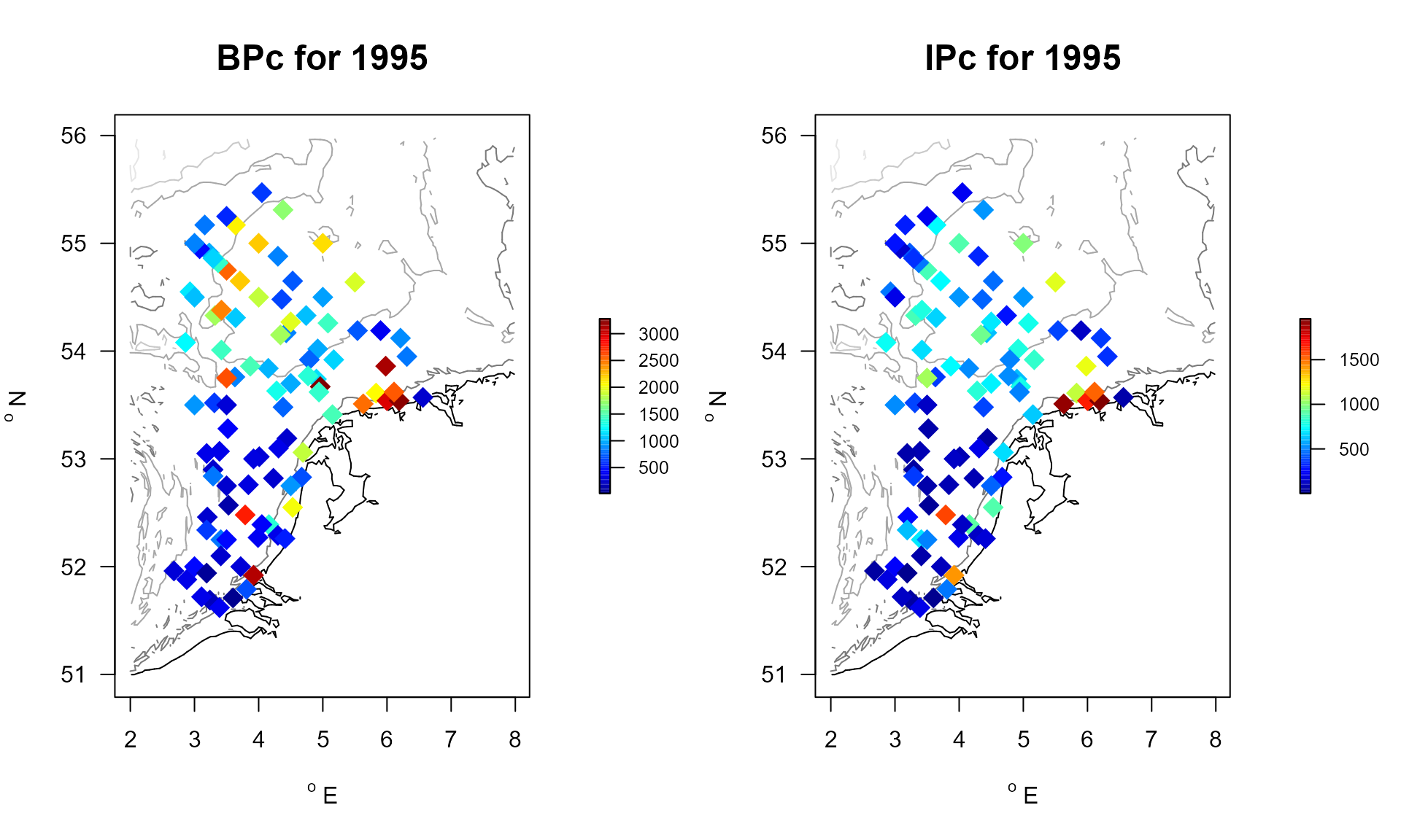
References

R-packages and data sources

R Core Team (2022). R: A Language and Environment for Statistical Computing. R Foundation for Statistical Computing, Vienna, Austria. https://www.R-project.org/.

Soetaert K (2021). plot3D: Plotting Multi-Dimensional Data. R package version 1.4, https://CRAN.R-project.org/package=plot3D.

Soetaert K, Beauchard O (2023). Btrait: Working with Biological density, taxonomy, and trait composition data. R package version 0.0.0.

Holstein Jan (2018). worms: Retrieving Aphia Information from World Register of Marine Species. R package version 0.2.2. https://CRAN.R-project.org/package=worms

EMODnet Biology (2022) Full Occurrence Data and Parameters downloaded from the EMODnet Biology project, consulted on 2022-08-05.

Beauchard O, Brind’Amour A, Schratzberger M, Laffargue P, Hintzen NT, Somerfield PJ, Piet G (2021) A generic approach to develop a trait-based indicator of trawling-induced disturbance. Mar Ecol Prog Ser 675:35-52. https://doi.org/10.3354/meps13840

Olivier Beauchard, Kari Elsa Ellingsen, Murray S.A. Thompson, Gerjan Piet, Pascal Laffargue, Karline Soetaert, in press. Assessing sea floor functional diversity and vulnerability. Marine Ecology Progress Series

Clare, David S. / Bolam, Stefan G. / McIlwaine, Paul S.O. / Garcia, Clement / Murray, Joanna M. / Eggleton, Jacqueline D. (2022). Ten key biological traits of marine benthic invertebrates surveyed in Northwest Europe. Cefas, UK. V2. doi: https://doi.org/10.14466/CefasDataHub.123

Heip, C.H.R.; Basford, D.; Craeymeersch, J.A.; Dewarumez, J.-M.; Dorjes, J.; de Wilde, P.; Duineveld, G.; Eleftheriou, A.; Herman, P.M.J.; Kingston, K.; Niermann, U.; Kunitzer, A.; Rachor, E.; Rumohr, H.; Soetaert, K.; Soltwedel, T. (1992). Trends in biomass, density and diversity of North Sea macrofauna. ICES J. Mar. Sci./J. Cons. int. Explor. Mer 49: 13-22

L. Leewis, E.C. Verduin, R. Stolk, 2017. Eurofins AquaSense Macrozoobenthosonderzoek in de Rijkswateren met boxcorer, jaarrapportage MWTL 2015 : waterlichaam: Noordzee. Publicatiedatum: 31-03-2017, 75 p. Projectnummer Eurofins AquaSense: J00002105, Revisie 2; In opdracht van Ministerie van Infrastructuur en Milieu, Rijkswaterstaat Centrale Informatievoorziening (RWS, CIV)

Queiros, Ana M., Silvana N. R. Birchenough, Julie Bremner, Jasmin A. Godbold, Ruth E. Parker, Alicia Romero-Ramirez, Henning Reiss, Martin Solan, Paul J. Somerfield, Carl Van Colen, Gert Van Hoey, Stephen Widdicombe, 2013. A bioturbation classification of European marine infaunal invertebrates. Ecology and Evolution 3 (11), 3958-3985

Solan M, Cardinale BJ, Downing AL, Engelhardt KAM, Ruesink JL, Srivastava DS. 2004. Extinction and ecosystem function in the marine benthos. Science 306:1177–80.

Wilson, R. J., Speirs, D. C., Sabatino, A., and Heath, M. R. (2018). A synthetic map of the north-west European Shelf sedimentary environment for applications in marine science. Earth Sys. Sci. Data 10, 109–130. doi: 10.5194/essd-10-109-2018

A. Wrede, J.Beermann, J.Dannheim, L.Gutow, T.Brey, 2018. Organism functional traits and ecosystem supporting services – A novel approach to predict bioirrigation. Ecological indicators, 91, 737-743.

Appendix

Description of the MWTL dataset

contents of data.frame ‘stations’ from the MWTL data
name	description	format
x	degrees longitude	WGS84
y	degrees latitude	WGS84

contents of data.frame ‘density’ from the MWTL data
name	description	units
station	station name
date	sampling date, a string
taxon	taxon name, checked by worms, and adjusted
density	species total density	individuals/m2
biomass	species total ash-free dry weight	gAFDW/m2
taxon.original	original taxon name

contents of data.frame ‘abiotics’ from the MWTL data
name	description	units
depth	water depth	m
D50	Median grain size	micrometer
mud	mud fraction (<63 um)	-
sand	sand fraction (64 -2000 um)	-
gravel	gravel fraction (>2000 um)	-
salinity	salinity
porosity	volumetric water content	-
permeability	permeability	m2
POC	particulate organic C in sediment	%
TN	total N in sediment	%
surfaceCarbon	particulate organic C in upper cm	%
surfaceNitrogen	total N in upper cm	%
orbitalVelMean	mean orbital velocity	m/s
orbitalVelMax	maximal orbital velocity	m/s
tidalVelMean	mean tidal velocity	m/s
tidalVelMax	maximal tidal velocity	m/s
bedstress	bed shear stress	Pa
EUNIScode	EUNIScode	-
SAR	swept area ratio (fisheries)	m2/m2/year

contents of data.frame ‘sediment’ from the MWTL data
name	description	units
D50	median grain size, in micrometer	micrometer
Silt	Silt+Clay fraction (< 63 micrometer) in %	%

contents of data.frame ‘fishing’ from the MWTL data
var	metadata.NIOZdata.fishing.	units
p0	proportion living ON sediment	-
p0_5cm	proportion living in upper 5 cm of the sediment, [0,1]	-
p5_15cm	proportion living in 5-15cm depth slice	-
p15_30cm	proportion living in 15-30cm depth slice	-
p30cm	proportion living in >30cm depth slice	-
swim	proportion swimmers	-
Life.span	longevity, years	years
r	rate of increase, estimated as 5.31/lifespan	/year

Description of the NSBS dataset

contents of data.frame ‘stations’ from the NSBS data
name	description	format
x	degrees longitude	WGS84
y	degrees latitude	WGS84

contents of data.frame ‘density’ from the NSBS data
name	description	units
station	station name
date	sampling date, a string
taxon	taxon name, checked by worms, and adjusted
density	species total density	individuals/m2

contents of data.frame ‘abiotics’ from the NSBS data
name	description	units
depth	water depth	m
D50	Median grain size	micrometer
mud	mud fraction (<63 um)	-
sand	sand fraction (64 -2000 um)	-
gravel	gravel fraction (>2000 um)	-
salinity	salinity
porosity	volumetric water content	-
permeability	permeability	m2
POC	particulate organic C in sediment	%
TN	total N in sediment	%
surfaceCarbon	particulate organic C in upper cm	%
surfaceNitrogen	total N in upper cm	%
orbitalVelMean	mean orbital velocity	m/s
orbitalVelMax	maximal orbital velocity	m/s
tidalVelMean	mean tidal velocity	m/s
tidalVelMax	maximal tidal velocity	m/s
bedstress	bed shear stress	Pa
EUNIScode	EUNIScode	-
SAR	swept area ratio (fisheries)	m2/m2/year

contents of data.frame ‘fishing’ from the NSBS data
var	metadata.NIOZdata.fishing.	units
p0	proportion living ON sediment	-
p0_5cm	proportion living in upper 5 cm of the sediment, [0,1]	-
p5_15cm	proportion living in 5-15cm depth slice	-
p15_30cm	proportion living in 15-30cm depth slice	-
p30cm	proportion living in >30cm depth slice	-
swim	proportion swimmers	-
Life.span	longevity, years	years
r	rate of increase, estimated as 5.31/lifespan	/year

Traits and modalities in the NIOZ database Traits

Effect traits, modalities, values and scores in the NIOZ database
colname	trait	modality	indic	value	score	units
ET1.M1	Substratum depth distribution	0	1	0.00	1.00	cm
ET1.M2	Substratum depth distribution	0-5	1	2.50	0.75	cm
ET1.M3	Substratum depth distribution	5-15	1	10.00	0.50	cm
ET1.M4	Substratum depth distribution	15-30	1	22.50	0.25	cm
ET1.M5	Substratum depth distribution	>30	1	30.00	0.00	cm
ET2.M1	Biodiffusion	Null	2	0.00	0.00	-
ET2.M2	Biodiffusion	Low	2	0.50	0.50	-
ET2.M3	Biodiffusion	High	2	1.00	1.00	-
ET3.M1	Downward conveying	Null	3	0.00	0.00	-
ET3.M2	Downward conveying	Low	3	0.50	0.50	-
ET3.M3	Downward conveying	High	3	1.00	1.00	-
ET4.M1	Upward conveying	Null	4	0.00	0.00	-
ET4.M2	Upward conveying	Low	4	0.50	0.50	-
ET4.M3	Upward conveying	High	4	1.00	1.00	-
ET5.M1	Regeneration	Null	5	0.00	0.00	-
ET5.M2	Regeneration	Low	5	0.50	0.50	-
ET5.M3	Regeneration	High	5	1.00	1.00	-
ET6.M1	Biodeposition	Null	6	0.00	0.00	-
ET6.M2	Biodeposition	Low	6	0.50	0.50	-
ET6.M3	Biodeposition	High	6	1.00	1.00	-
ET7.M1	Bioerosion	Null	7	0.00	0.00	-
ET7.M2	Bioerosion	Low	7	0.50	0.50	-
ET7.M3	Bioerosion	High	7	1.00	1.00	-
ET8.M1	Biostabilisation	Null	8	0.00	0.00	-
ET8.M2	Biostabilisation	Low	8	0.50	0.50	-
ET8.M3	Biostabilisation	High	8	1.00	1.00	-
ET9.M1	Ventilation/Pumping	Null	9	0.00	0.00	-
ET9.M2	Ventilation/Pumping	Low	9	0.50	0.50	-
ET9.M3	Ventilation/Pumping	High	9	1.00	1.00	-
ET10.M1	Burrow width	None	10	0.00	0.00	mm
ET10.M2	Burrow width	Narrow	10	5.00	0.33	mm
ET10.M3	Burrow width	Intermediate	10	7.50	0.67	mm
ET10.M4	Burrow width	Wide	10	12.50	1.00	mm
ET11.M1	Endo-3D structure type	None	11	0.00	0.00	-
ET11.M2	Endo-3D structure type	Chimney/Funnel	11	0.17	0.17	-
ET11.M3	Endo-3D structure type	Tube	11	0.33	0.33	-
ET11.M4	Endo-3D structure type	IJ-shaped burrow	11	0.50	0.50	-
ET11.M5	Endo-3D structure type	UY-shaped burrow	11	0.67	0.67	-
ET11.M6	Endo-3D structure type	Branched burrow	11	0.83	0.83	-
ET11.M7	Endo-3D structure type	Anastomosed burrow	11	1.00	1.00	-
ET12.M1	Endo-3D structure depth	None	12	0.00	0.00	cm
ET12.M2	Endo-3D structure depth	0-5	12	2.50	0.25	cm
ET12.M3	Endo-3D structure depth	5-15	12	10.00	0.50	cm
ET12.M4	Endo-3D structure depth	15-30	12	22.50	0.75	cm
ET12.M5	Endo-3D structure depth	>30	12	30.00	1.00	cm
ET13.M1	Epi-3D structure type	None	13	0.00	0.00	-
ET13.M2	Epi-3D structure type	Mat	13	0.17	0.17	-
ET13.M3	Epi-3D structure type	Mound	13	0.33	0.33	-
ET13.M4	Epi-3D structure type	Tube/Tubular protrusion	13	0.50	0.50	-
ET13.M5	Epi-3D structure type	Shell	13	0.67	0.67	-
ET13.M6	Epi-3D structure type	Stalk/Feather	13	0.83	0.83	-
ET13.M7	Epi-3D structure type	Protuberance	13	1.00	1.00	-
ET14.M1	Epi-3D structure extension	None	14	0.00	0.00	-
ET14.M2	Epi-3D structure extension	Isolated/Clumped	14	0.25	0.25	-
ET14.M3	Epi-3D structure extension	Mat/Lawn	14	0.50	0.50	-
ET14.M4	Epi-3D structure extension	Simple reef	14	0.75	0.75	-
ET14.M5	Epi-3D structure extension	Complex reef	14	1.00	1.00	-
ET15.M1	Epi-3D structure size	None	15	0.00	0.00	mm
ET15.M2	Epi-3D structure size	<1	15	1.00	0.17	mm
ET15.M3	Epi-3D structure size	1-3	15	2.00	0.33	mm
ET15.M4	Epi-3D structure size	3-10	15	6.50	0.50	mm
ET15.M5	Epi-3D structure size	10-20	15	15.00	0.67	mm
ET15.M6	Epi-3D structure size	20-50	15	35.00	0.83	mm
ET15.M7	Epi-3D structure size	>50	15	50.00	1.00	mm

Response traits, modalities, values and scores in the NIOZ database
colname	trait	modality	indic	value	score	units
RT1.M1	Body mass	<0.001	1	0.00e+00	0.00	gADWt
RT1.M2	Body mass	0.001-0.010	1	0.00e+00	0.25	gADWt
RT1.M3	Body mass	0.010-0.100	1	5.00e-02	0.50	gADWt
RT1.M4	Body mass	0.100-1.000	1	5.00e-01	0.75	gADWt
RT1.M5	Body mass	>1.000	1	5.00e+00	1.00	gADWt
RT2.M1	Body length	<1	2	5.00e-01	0.00	mm
RT2.M2	Body length	1-3	2	2.00e+00	0.25	mm
RT2.M3	Body length	3-10	2	6.50e+00	0.50	mm
RT2.M4	Body length	10-20	2	1.50e+01	0.75	mm
RT2.M5	Body length	20-50	2	3.50e+01	1.00	mm
RT3.M1	Body resistance	Very low	3	0.00e+00	1.00	-
RT3.M2	Body resistance	Low	3	2.50e-01	0.75	-
RT3.M3	Body resistance	Intermediate	3	5.00e-01	0.50	-
RT3.M4	Body resistance	High	3	7.50e-01	0.25	-
RT3.M5	Body resistance	Very high	3	1.00e+00	0.00	-
RT4.M1	Motility	Sessile	4	0.00e+00	1.00	-
RT4.M2	Motility	Tubicolous	4	3.30e-01	0.67	-
RT4.M3	Motility	Crawler	4	6.70e-01	0.33	-
RT4.M4	Motility	Swimmer	4	1.00e+00	0.00	-
RT5.M1	Burrowing/Sheltering depth	0	5	0.00e+00	1.00	cm
RT5.M2	Burrowing/Sheltering depth	0-5	5	2.50e+00	0.75	cm
RT5.M3	Burrowing/Sheltering depth	5-15	5	1.00e+01	0.50	cm
RT5.M4	Burrowing/Sheltering depth	>15	5	2.00e+01	0.25	cm
RT6.M1	Feeding type	Deposit feeder	6	0.00e+00	0.00	-
RT6.M2	Feeding type	Suspension feeder	6	3.30e-01	0.33	-
RT6.M3	Feeding type	Herbivore/Grazer	6	6.70e-01	0.67	-
RT6.M4	Feeding type	Carnivore/Scavenger	6	1.00e+00	1.00	-
RT7.M1	Life span	<1	7	5.00e-01	0.00	year
RT7.M2	Life span	1-3	7	2.00e+00	0.25	year
RT7.M3	Life span	3-10	7	6.50e+00	0.50	year
RT7.M4	Life span	10-20	7	1.50e+01	0.75	year
RT7.M5	Life span	>20	7	3.00e+01	1.00	year
RT8.M1	Age at maturity	<1	8	5.00e-01	0.00	year
RT8.M2	Age at maturity	1-3	8	2.00e+00	0.50	year
RT8.M3	Age at maturity	3-5	8	4.00e+00	1.00	year
RT9.M1	Reproductive frequency	Sexual seasonal	9	0.00e+00	0.00	-
RT9.M2	Reproductive frequency	Sexual continuous	9	1.00e+00	1.00	-
RT10.M1	Fertilisation	Broadcasting	10	0.00e+00	0.00	-
RT10.M2	Fertilisation	Spermcasting	10	5.00e-01	0.50	-
RT10.M3	Fertilisation	Pairing	10	1.00e+00	1.00	-
RT11.M1	Annual fecundity	<10e2	11	5.00e+01	0.00	-
RT11.M2	Annual fecundity	10e2-10e3	11	4.50e+02	0.20	-
RT11.M3	Annual fecundity	10e3-10e4	11	4.50e+03	0.40	-
RT11.M4	Annual fecundity	10e4-10e5	11	4.50e+04	0.60	-
RT11.M5	Annual fecundity	10e5-10e6	11	4.50e+05	0.80	-
RT11.M6	Annual fecundity	>10e6	11	1.00e+06	1.00	-
RT12.M1	Offspring type	Egg	12	0.00e+00	0.00	-
RT12.M2	Offspring type	Larva	12	5.00e-01	0.50	-
RT12.M3	Offspring type	Juvenile	12	1.00e+00	1.00	-
RT13.M1	Offspring size	<0.1	13	5.00e-02	0.00	mm
RT13.M2	Offspring size	0.1-0.5	13	3.00e-01	0.33	mm
RT13.M3	Offspring size	0.5-1.5	13	1.00e+00	0.67	mm
RT13.M4	Offspring size	1.5-5	13	3.25e+00	1.00	mm
RT14.M1	Offspring protection	None	14	0.00e+00	0.00	-
RT14.M2	Offspring protection	Gel	14	2.50e-01	0.25	-
RT14.M3	Offspring protection	Capsule	14	5.00e-01	0.50	-
RT14.M4	Offspring protection	Burrying	14	7.50e-01	0.75	-
RT14.M5	Offspring protection	Bearing/Brooding	14	1.00e+00	1.00	-
RT15.M1	Offspring development	Planktotrophic	15	0.00e+00	0.00	-
RT15.M2	Offspring development	Lecithotrophic	15	2.50e-01	0.25	-
RT15.M3	Offspring development	Mixed planktotrophic	15	5.00e-01	0.50	-
RT15.M4	Offspring development	Mixed lecithotrophic	15	7.50e-01	0.75	-
RT15.M5	Offspring development	Internal	15	1.00e+00	1.00	-
RT16.M1	Offspring benthic stage duration	Null	16	0.00e+00	0.00	days
RT16.M2	Offspring benthic stage duration	<15	16	7.50e+00	0.25	days
RT16.M3	Offspring benthic stage duration	15-30	16	2.25e+01	0.50	days
RT16.M4	Offspring benthic stage duration	30-60	16	4.50e+01	0.75	days
RT16.M5	Offspring benthic stage duration	>60	16	6.00e+01	1.00	days
RT17.M1	Offspring pelagic stage duration	Null	17	0.00e+00	0.00	days
RT17.M2	Offspring pelagic stage duration	<15	17	7.50e+00	0.25	days
RT17.M3	Offspring pelagic stage duration	15-30	17	2.25e+01	0.50	days
RT17.M4	Offspring pelagic stage duration	30-60	17	4.50e+01	0.75	days
RT17.M5	Offspring pelagic stage duration	>60	17	6.00e+01	1.00	days

Traits and modalities in the CEFAS database Traits_cefas

Effect traits, modalities, values and scores in Traits_cefas
colname	trait	modality	indic	value	score
sr_Less_than_10	Maximum size	<10	1	5.00	0.00
sr_11_to_20	Maximum size	11-20	1	15.00	0.20
sr_21_to_100	Maximum size	21-100	1	60.00	0.40
sr_101_to_200	Maximum size	101-200	1	150.00	0.60
sr_201_to_500	Maximum size	201-500	1	350.00	0.80
sr_More_than_500	Maximum size	>500	1	750.00	1.00
m_Soft	Morphology	Soft	2	0.00	0.00
m_Tunic	Morphology	Tunic	2	0.20	0.20
m_Exoskeleton	Morphology	Exoskeleton	2	0.40	0.40
m_Crustose	Morphology	Crustose	2	0.60	0.60
m_Cushion	Morphology	Cushion	2	0.80	0.80
m_Stalked	Morphology	Stalked	2	1.00	1.00
l_Less_than_1	Lifespan	<1	3	0.50	0.00
l_1_to_3	Lifespan	1-3	3	2.00	0.33
l_3_to_10	Lifespan	3-10	3	6.50	0.67
l_More_than_10	Lifespan	>10	3	15.00	1.00
ed_Asexual	Egg development location	Asexual	5	0.00	0.00
ed_Sexual_pelagic	Egg development location	Sexual_pelagic	5	0.33	0.33
ed_Sexual_benthic	Egg development location	Sexual_benthic	5	0.67	0.67
ed_Sexual_brooded	Egg development location	Sexual_brooded	5	1.00	1.00
ld_Pelagic_planktotrophic	Larva development location	Pelagic_planktotrophic	6	0.00	0.00
ld_Pelagic_lecithotrophic	Larva development location	Pelagic_lecithotrophic	6	0.50	0.50
ld_Benthic_direct	Larva development location	Benthic_direct	6	1.00	1.00
lh_Tube_dwelling	Living habit	Tube_dwelling	7	0.00	0.00
lh_Burrow_dwelling	Living habit	Burrow_dwelling	7	0.20	0.20
lh_Free_living	Living habit	Free_living	7	0.40	0.40
lh_Crevice_hole_under_stones	Living habit	Crevice_hole_under_stones	7	0.60	0.60
lh_Epi_endo_biotic	Living habit	Epi_endo_biotic	7	0.80	0.80
lh_Attached_to_substratum	Living habit	Attached_to_substratum	7	1.00	1.00
sp_Surface	Sediment position	Surface	8	0.00	0.00
sp_Shallow_infauna_0_to_5cm	Sediment position	Shallow_infauna_0_to_5cm	8	2.50	0.33
sp_Mid_depth_infauna_5_to_10cm	Sediment position	Mid_depth_infauna_5_to_10cm	8	7.50	0.67
sp_Deep_infauna_more_than_10cm	Sediment position	Deep_infauna_more_than_10cm	8	15.00	1.00
f_Suspension	Feeding mode	Suspension	9	0.00	0.00
f_Surface_deposit	Feeding mode	Surface_deposit	9	0.20	0.20
f_Subsurface_deposit	Feeding mode	Subsurface_deposit	9	0.40	0.40
f_Scavenger	Feeding mode	Scavenger	9	0.60	0.60
f_Predator	Feeding mode	Predator	9	0.80	0.80
f_Parasite	Feeding mode	Parasite	9	1.00	1.00
mob_Sessile	Mobility	Sessile	10	0.00	0.00
mob_Swim	Mobility	Swim	10	0.33	0.33
mob_Crawl_creep_climb	Mobility	Crawl_creep_climb	10	0.67	0.67
mob_Burrower	Mobility	Burrower	10	1.00	1.00
b_Diffusive_mixing	Bioturbation mode	Diffusive_mixing	11	0.00	0.00
b_Surface_deposition	Bioturbation mode	Surface_deposition	11	0.25	0.25
b_Upward_conveyor	Bioturbation mode	Upward_conveyor	11	0.50	0.50
b_Downward_conveyer	Bioturbation mode	Downward_conveyer	11	0.75	0.75
b_None	Bioturbation mode	None	11	1.00	1.00

Traits and modalities in the bioturbation database Traits_Db

Effect traits, modalities, values and scores in Traits_Db
trait	modality	description
Ri	1	epifauna
Ri	2	surficial modifiers
Ri	3	upward and downward conveyors
Ri	4	biodiffusors
Ri	5	regenerators
Mi	1	organisms that live in fixed tubes
Mi	2	limited movement
Mi	3	slow, free movement through the sediment matrix
Mi	4	free movement, via burrow system
Fti	S	surficial modifiers
Fti	B	biodiffusors
Fti	UC	upward conveyors
Fti	DC	downward conveyors
Fti	R	regenerators
Fti	E	epifauna

Traits and modalities in the bioirrigation database Traits_irr

Effect traits, modalities, values and scores in Traits_irr
trait	modality	description
BT	1	epifauna, internal irrigation (e.g. siphons)
BT	2	open irrigation (e.g. U- or Y- shaped burrows)
BT	3	blind ended irrigation
ID	1	injection pocket 0-2cm
ID	2	injection pocket 2-5cm
ID	3	injection pocket 5-10cm
ID	4	injection pocket >10 cm depth
FT	1	surface filter feeders
FT	2	predators
FT	3	deposit feeders
FT	4	sub surface filter feeders

Karline Soetaert and Olivier Beauchard

18 November 2022