The Bfiat package: modelling trawling effects in the Dutch part of the Northsea

Karline Soetaert and Olivier Beauchard

Abstract

The impact of bottom trawling on benthic life in the Dutch part of the Northsea is estimated. We use monitoring data from 103 stations in the area (MWTL data set), and impose fishing intensities estimated for each of these stations.

Aim.

We use functions from the Btrait and Bfiat R-packages to estimate the impact of bottom fisheries on sediment ecosystem functioning in the Dutch part of the Northsea.

We use three sets of data:

• in situ density data from a particular site.
• species trait information, including:
  • the age at maturity of the species, and
  • the depth of occurrence in the sediment.
• fishing intensity and gear penetration depths in the sites

We use the MWTL macrofauna density data that have been compiled in the frame of the EMODnet biology project, (https://www.emodnet-biology.eu). These data are available from the R-package Btrait (Soetaert and Beauchard, 2024a).

The NIOZ trait database is used for the species traits (Beauchard et al., 2021, 2023). The trait dataset is also in the R-package Btrait.

Software.

The fishing impact models run in the open source framework R (R core team, 2025) and have been implemented in the Bfiat R-package (Soetaert and Beauchard, 2024b).

The R-package Btrait (Soetaert and Beauchard, 2022) contains functions to work on density and trait datasets.

The packages Btrait and Bfiat are available on github (https://github.com/EMODnet/Btrait and https://github.com/EMODnet/Bfiat).

The fisheries impact model

The fisheries impact model is based on the logistic growth equation (Verhulst 1845) that describes how species density or biomass evolves over time. The effect of fishing on the population is included as a series of events, that instantaneously decimate population sizes, while in between these events the populations recover.

The model thus consists of two parts: (continuous) logistic growth in between fishing events and an instantaneous depletion during fishing.

Logistic growth

The differential equation is, for t in between $t_j^+$ and $t_{j+1}^-$: $$\frac{dD_i^t}{dt}=r_i \cdot D_i^t \cdot (1-\frac{D_i^t}{K_i}),$$ where $t$ is time, $D_i^t$ is the density of species $i$ at a particular time, $K_i$ (units of density) is the carrying capacity of species $i$, $r_i$ is the logistic growth parameter (units [/time]).

Instantaneous trawling

During trawling at times $t_j$, density changes instantaneously:

$$D_i^{t_j^+} = D_i^{t_j^-} \cdot (1-d_i),$$

where $D_i^{t_j^+}$ and $D_i^{t_j^-}$ are the density immediately after and before trawling occurs at time $t_j$ respectively, and $d_i$ is the species-specific and trawl-specific depletion fraction.

Trawling intensity

The time in between trawling can be inferred from the fishing intensity, expressed as the annual swept area ratio (SAR).

SAR is the cumulative area contacted by a fishing gear over one year and per surface area. It has units of $m^2~m^{-2}~yr^{-1}$, or $yr^{-1}$.

From the swept area ratio (hereafter denoted as $S$), we calculate the average time in between fishing events ($yr$) as:

$$\Delta t = t_{j+1} - t_j = \frac{1}{S}.$$

Data requirements

Central in the impact analysis is the use of a combination of data sets:

Community composition

Benthic biological data to be used for fishing assessment should comprise at least density data, and preferentially also biomass of individual species.

The densities or biomasses are used to estimate the “carrying capacity” of the species at a particular site; this is the abundance the species attains at steady-state, when undisturbed (i.e. in the absence of fishing).

Taxonomy

To assign biological traits to the taxa in the community, it is convenient to know their taxonomic position. Thus it will be possible to derive trait characteristics for taxa that are not documented in the trait database, based on their taxonomic relationships.

Trait characteristics

The following species traits are used to estimate the fishing impact on species density:

• The age at maturity of species is used to estimate their “intrinsic rate of natural increase” ($r_i$).
• The depth at which species live determines their vulnerability to bottom trawling: it is used to derive the model’s “depletion parameter” ($d_i$).

Fishing intensity

The model also needs the fishing intensity for a certain area, for instance expressed as the annual swept area ratio (SAR); this is the cumulative area contacted by a fishing gear over one year and per surface area.

From the swept area ratio (hereafter denoted as $S$, units $yr^{-1}$), we calculate the time in between fishing events ($yr$) as $\frac{1}{S}$.

Data availability

Community composition

For the subsequent analyses, we use macrofauna density data that have been compiled in the frame of the EMODnet biology project, (https://www.emodnet-biology.eu).

The monitoring data from the Dutch part of the North sea (called the MWTL monitoring data) comprise both species densities and biomass for 103 stations, that were sampled during 19 years, extending from 1995 till 2018.

Sampling was performed yearly at first, then less frequently. Calculations in this document are based on yearly averages.

The MWTL data are available from the R-package Btrait, and are in a list called MWTL (within R, type: ?MWTL to open the help file for these data).

The composition of the MWTL data is in Appendix 1.

TABLE: Metadata of the MWTL dataset

title	originator	implemented
The MWTL Northsea macrobenthos data (1995 - 2018)	Ministerie van Infrastructuur en Milieu, Rijkswaterstaat Centrale Informatievoorziening (RWS, CIV)	Karline Soetaert, in the frame of the EMODnet biology project

TABLE: MWTL$density (first 3 rows)

station	date	year	taxon	density	biomass
BREEVTN02	27-06-1995	1995	Bathyporeia guilliamsoniana	14.6	0.0044
BREEVTN02	27-06-1995	1995	Callianassa	58.5	1.3986
BREEVTN02	27-06-1995	1995	Chaetozone setosa	14.6	0.0073

Taxonomic data

There are 400 different taxa in the MWTL data.

The taxonomic information for all taxa, has been derived from the WoRMS database and is available from package Btrait, in dataset Taxonomy:

TABLE: Dataset Taxonomy (first 3 rows)

taxon	genus	family	order	class	phylum	AphiaID
Abietinaria	Abietinaria	Sertulariidae	Leptothecata	Hydrozoa	Cnidaria	117225
Abludomelita	Abludomelita	Melitidae	Amphipoda	Malacostraca	Arthropoda	101665
Abludomelita obtusata	Abludomelita	Melitidae	Amphipoda	Malacostraca	Arthropoda	102788

Trait data

We use the traits compiled by NIOZ (called Traits_nioz) for age at maturity, and living depth. These trait data (mainly on species level) were compiled by Beauchard et al. (2021) and Beauchard et al. (2023). This database records 32 different traits from 281 taxa.

All traits are fuzzy-coded. The data structure is in appendix 2.

TABLE: First part of dataset Traits_nioz

taxon	ET1.M1	ET1.M2	ET1.M3	ET1.M4
Abludomelita	0.5	0.5	0.0	0
Abludomelita obtusata	0.5	0.5	0.0	0
Abra alba	0.0	0.5	0.5	0

The figure below shows the position and area of the MWTL stations, and the swept area ratios (sar) that were derived from OSPAR (ICES 2018).

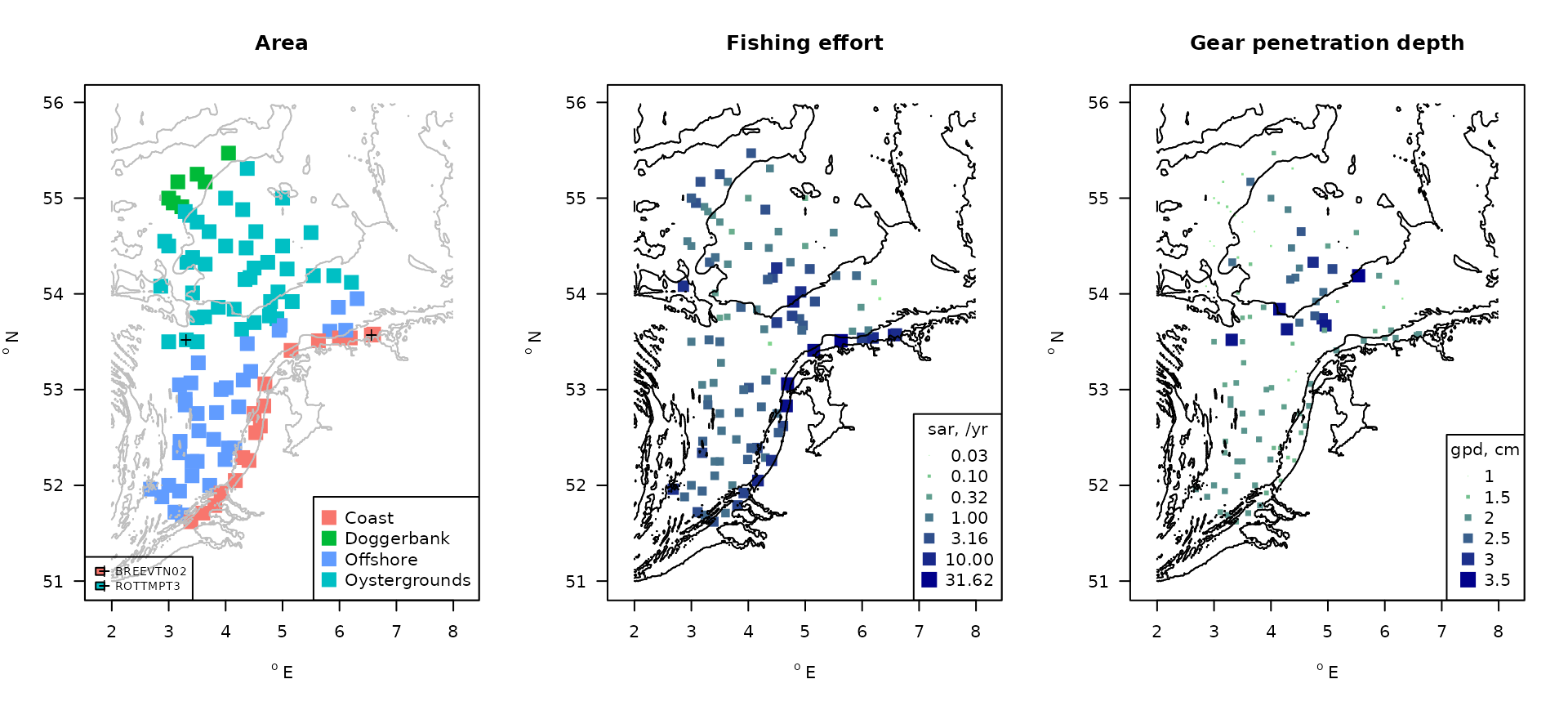
FIG: MWTL sampling stations with indication of the main areas, fishing intensity and gear penetration depth. ‘+’ denote the two stations that will be showcased.

Model steps

The model is applied in several steps:

• the taxon densities per station are prepared, and a list of taxa in the data is generated,
• the traits recording age at maturity and the depth distribution for each taxon are extracted,
• the fishing parameters for each station are extracted
• the parameter values are estimated based on the traits, fishing parameters, and taxon density
• the model is run

The MWTL density

The MWTL data are gathered over several years, and are in data.frame MWTL$density. We calculate the density for all stations (descriptor) and taxa, averaged over all years, using Btrait function get_density.

MeanMWTL <- 
  get_density(data        = MWTL$density,
              descriptor  = station,  
              taxon       = taxon,
              value       = density,
              averageOver = year)

The taxa whose traits need to be found are extracted:

MWTLtaxa <- sort(unique(MeanMWTL$taxon))  

Extracting taxon traits

Taxon traits that we need are in the nioz trait database (Traits_nioz), from R-package Btrait. From this database, we use:

• the depth distribution (fractional occurrence in each depth layer),
• the age at maturity of a species

Substrate depth distribution

Depth distribution is a fuzzy-coded trait in the trait database. For use in the model we need to keep it fuzzy coded.

The meaning of the nioz traits is stored in its metadata. We look for the trait names that relate to depth distribution:

meta   <- metadata(Traits_nioz)  # description of trait modalities

meta.D <- subset(meta,           # names of trait modalities for substratum depth
                 subset = (trait == "Substratum depth distribution"))

TABLE: Depth distribution traits in the NIOZ trait database

colname	trait	modality	indic	value	score	units
ET1.M1	Substratum depth distribution	0	1	0.0	1.00	cm
ET1.M2	Substratum depth distribution	0-5	1	2.5	0.75	cm
ET1.M3	Substratum depth distribution	5-15	1	10.0	0.50	cm
ET1.M4	Substratum depth distribution	15-30	1	22.5	0.25	cm
ET1.M5	Substratum depth distribution	>30	1	30.0	0.00	cm

We then extract the depth traits for each taxon in the MWTL density data set. As not all species in the MWTL dataset have traits assigned, we use the taxonomic information (in dataset Taxonomy) to estimate the traits also for unrecorded species.

traits.D <- get_trait(
                taxon    = MWTLtaxa, 
                trait    = Traits_nioz[, c("taxon", meta.D$colname)], 
                taxonomy = Taxonomy)

colnames(traits.D)[-1] <- meta.D$modality     # suitable column names

TABLE: Depth distribution of species in the MWTL dataset, (first part)

taxon	0	0-5	5-15	15-30	>30
Abludomelita obtusata	0.5	0.5	0.0	0	0
Abra alba	0.0	0.5	0.5	0	0
Abra nitida	0.0	1.0	0.0	0	0

Of the 400 taxa in the MWTL dataset, only 209 taxa are documented in the trait database. The traits for the remaining taxa were estimated based on taxonomic closedness. Of these taxa, only 8 could not be assigned a trait. These were: Ascidiacea, Chaetognatha, Enteropneusta, Entoprocta, Nematoda, Nemertea, Platyhelminthes, Priapulida. As these taxa are not true macrofauna, they can be removed from the dataset.

Notrait  <- attributes(traits.D)$notrait
MWTLtaxa <- MWTLtaxa [! MWTLtaxa %in% Notrait]
MeanMWTL <- MeanMWTL [! MeanMWTL$taxon %in% Notrait, ]

Age at maturity

We perform a similar procedure to extract the age at maturity for each taxon in the density data. The age at maturity is estimated as the average of the fuzzy values.

We first find the relevant trait names in the trait database:

meta.A <- subset(meta,     
                 subset = (trait == "Age at maturity"))

TABLE: Age at maturity traits in the NIOZ trait database

colname	trait	modality	indic	value	score	units
RT8.M1	Age at maturity	<1	8	0.5	0.0	year
RT8.M2	Age at maturity	1-3	8	2.0	0.5	year
RT8.M3	Age at maturity	3-5	8	4.0	1.0	year

We then calculate the average age at maturity. To calculate the average, we pass the trait_class and trait_score while extracting the traits.

traits.A <- get_trait( 
               taxon       = MWTLtaxa, 
               trait       = Traits_nioz[, c("taxon", meta.A$colname)], 
               trait_class = meta.A$trait, 
               trait_score = meta.A$value, 
               taxonomy    = Taxonomy)

TABLE: Mean age at maturity of species ([yr]) in the MWTL dataset (first part)

taxon	Age.at.maturity
Abludomelita obtusata	0.5
Abra alba	0.5
Abra nitida	0.5

Merged trait-density data.frame

We merge these two trait datasets in one data.frame, merging by the taxon.

TraitsAll <- merge(x  = traits.A, 
                   y  = traits.D, 
                   by = "taxon")

and then combine it with the species density data

MWTLtrait <- merge(x  = MeanMWTL, 
                   y  = TraitsAll,
                   by = "taxon")

Fishing parameters

Each station has a specific fishing intensity (swept area ratio, sar), and mean gear penetration depth (gpd). This information is kept in data.frame MWTL$abiotics (from R-package Btrait).

The MWTL data.frame are merged with the swept area ratio, and with the gear penetration depth, merging on column station.

MWTLtrait <- merge(x  = MWTLtrait, 
                   y  = subset(MWTL$abiotics, 
                               select = c(station, sar, gpd)),
                   by = "station")

Parameter values

Intrinsic rate of natural increase

The intrinsic rate of natural increase is specific for a species, and can be estimated using function par_r. This parameter is added to the MWTL data.frame.

MWTLtrait$r <- par_r(age_at_maturity = MWTLtrait$Age.at.maturity)

Depletion fraction d

The depletion rate depends on the depth occurrence of the species (fDepth), and on the gear penetration depth (gpd).

The latter differs among stations, so the species depletion fraction will vary with the station.

We also need to input the upper position of each depth layer (uDepth).

MWTLtrait$d <- par_d(
  gpd    = MWTLtrait$gpd,
  
  fDepth = MWTLtrait[, c( "0", "0-5", "5-15", "15-30", ">30")],
  uDepth =             c(   0,     0,     5,      15,    30)
)

Carrying capacity K

Te carrying capacity is estimated from the model itself. We pass the species density, the fishing intensity (sar), the rate of increase (r), and the depletion fraction (d):

MWTLtrait$K <- par_K(
  
  density = MWTLtrait$density,
  sar     = MWTLtrait$sar,
  
  r       = MWTLtrait$r,
  d       = MWTLtrait$d
)

The data that we will use for fishing impact assessment is:

TABLE: First part of data used for fishing assessment

station	taxon	r	d	K	sar	gpd
BREEVTN02	Ophiura	0.96	0.16	2.87	1.42	2.95
BREEVTN02	Sthenelais limicola	0.73	0.14	5.64	1.42	2.95
BREEVTN02	Diplocirrus glaucus	1.89	0.11	6.23	1.42	2.95

Species for which the model does not find a solution

These are species where the depletion is too high and/or the intrinsic rate of increase is too low, so that it cannot persist in the environment under the current fishing pressure. This causes an anomalously high carrying capacity compared to observed density. Such occurrences are removed from the data set.

MWTLtrait$DK <- MWTLtrait$density/MWTLtrait$K
ii <- which(is.na(MWTLtrait$DK)) 
NAS <- subset(MWTLtrait, subset = is.na(DK))

MWTLtrait <- MWTLtrait[-ii,]

There are 16 such species, the highest observed density being17.4415692. These taxa are removed from the analysis.

TT <- data.frame(table(NAS$taxon))
TM <- aggregate(NAS$density, list(NAS$taxon), FUN=max)
TT <- merge(TT, TM, by = 1)
names(TT) <- c("taxon", "occurrences", "max density")
knitr::kable(TT, caption = "Taxa for which the model could not be solved")

Taxa for which the model could not be solved

taxon	occurrences	max density
Amphiura filiformis	1	0.6747638
Astropecten	2	11.5504579
Crangon crangon	1	0.6747638
Cucumaria	1	0.6842105
Ensis ensis	1	2.4416667
Eteone longa	1	2.9852901
Eudorella truncatula	1	3.4690862
Kurtiella bidentata	1	7.0395316
Ophiura	2	4.0242915
Paraleptopentacta elongata	1	1.4431849
Pholoe baltica	1	5.4170040
Pholoe minuta	2	13.2036283
Spisula subtruncata	1	17.4415692

Running the fishing model

We run the model for 8255 species-station occurrences. The model is run for 30 years, of which 20 years of fishing (and thus 10 years where fishing stopped).

We provide taxon names to label the output columns

times <- seq(from = 0, to = 30, length.out = 3000)

system.time(
dens  <- density_perturb(parms        = MWTLtrait, 
                         times        = times, 
                         taxon_names  = paste(MWTLtrait$station, 
                                              MWTLtrait$taxon, sep = "_"),
                         tend_perturb = 20)
)

##    user  system elapsed 
##   0.481   0.070   0.551

The result is a matrix with 3000 rows and 8256 columns, the first of which contains the time, followed by the density trajectories of all species, and for all stations.

TABLE: First part of model output

times	BREEVTN02_Ophiura	BREEVTN02_Sthenelais limicola	BREEVTN02_Diplocirrus glaucus
0.00	2.87	5.64	6.23
0.01	2.87	5.64	6.23
0.02	2.87	5.64	6.23

Summaries

The total density per station is calculated as rowSums per station.

Dens  <- data.frame(dens[, -1])  # remove first column
Total <- sapply(split.default(Dens, MWTLtrait$station), # split in stations
                FUN = rowSums, na.rm = TRUE)            # take row sums

Then relative values are calculated by dividing all columns (MARGIN = 2) by their maximum (STATS).

Drel <- sweep(x      = Total, 
              MARGIN = 2, 
              STATS  = apply(Total,            # max of each column
                             MARGIN = 2, 
                             FUN    = max), 
              FUN    = "/")                    # divide by the max

Some results

We show the results for the 20 most abundant species in two stations.

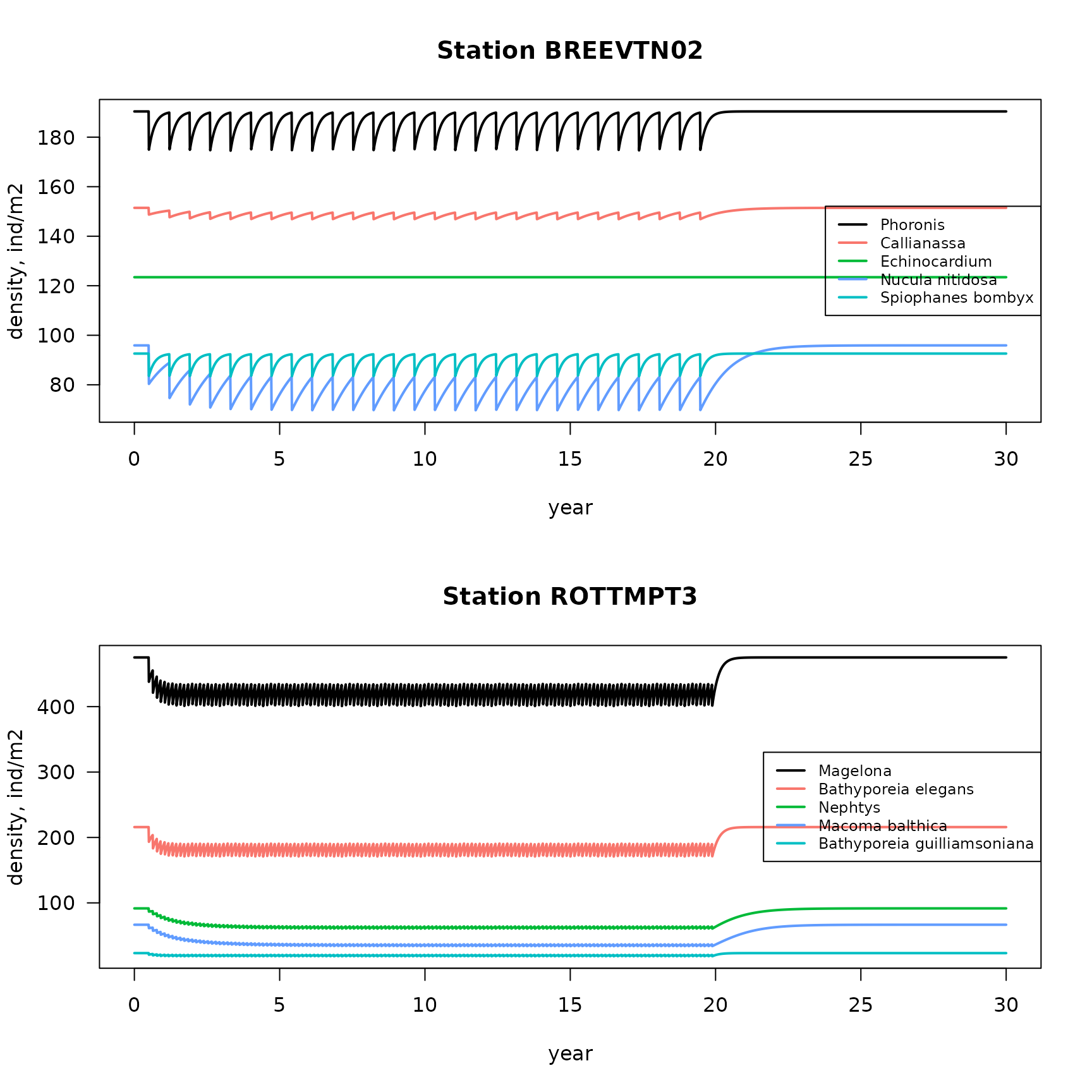
FIG: Density trajectories of 5 most abundant species from two stations

The average density reduction due to fishing in each of the stations is estimated:

# fishing reduction for all species
DDrel <- apply(X      = dens[, -1], 
               MARGIN = 2, 
               FUN    = function(x) 1-min(x)/max(x))

# averaged per station
DDstat <- aggregate(x   = list(p = DDrel), 
                    by  = list(station = MWTLtrait$station), 
                    FUN = mean)

MWTLstat <- merge(MWTL$stations, DDstat,   # add station coordinates 
                  by = "station")

with(MWTLstat, 
    map_MWTL(x    = x, y = y, colvar = p, 
             main = "Fractional reduction ", clab = "-", 
             col  = Colramp, cex = 2, pch = 15, log = "",
             type = "legend")
   )

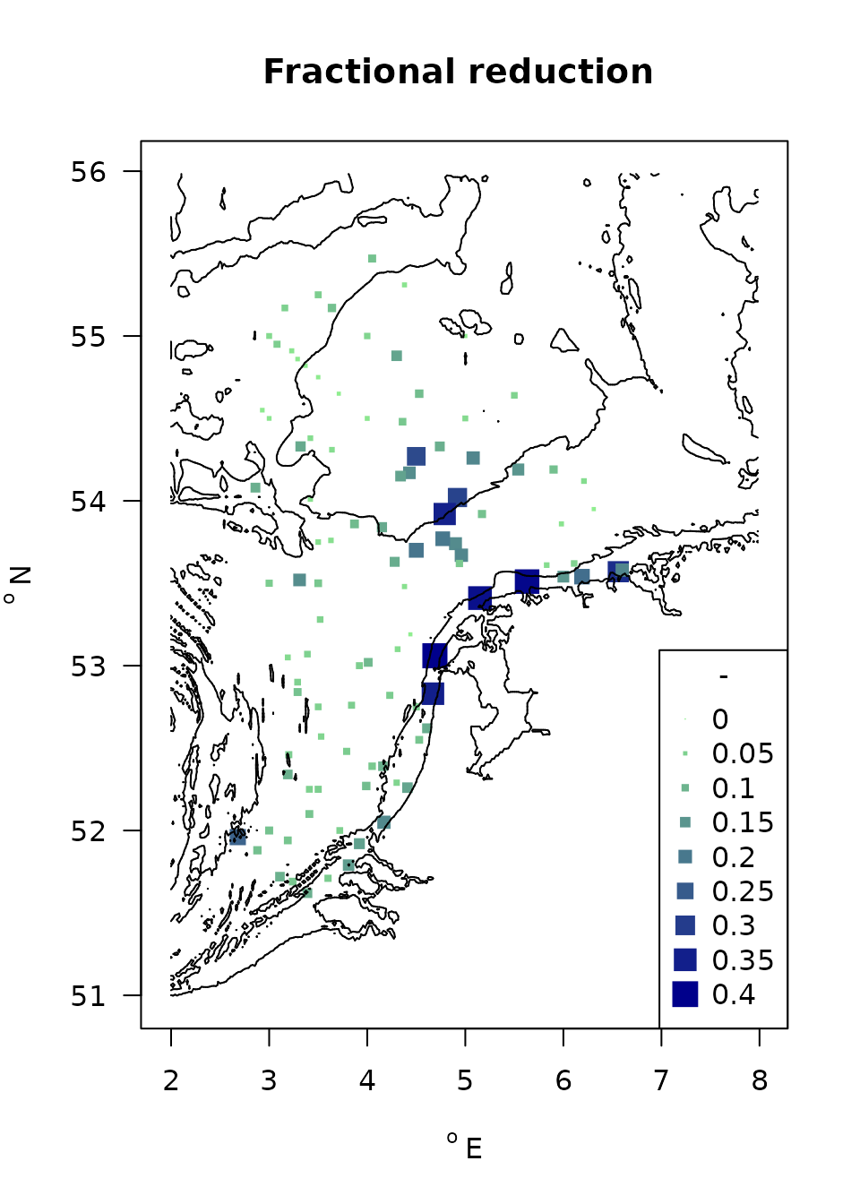
FIG: Average fishing impacts for the MWTL stations

Appendix

Structure of the MWTL data

The MWTL list contains several data.frames. We will use mainly the data.frames called density, stations, and abiotics (for fishing intensities). The structure of these data is:

TABLE: MWTL$station

name	description	format
x	degrees longitude	WGS84
y	degrees latitude	WGS84

TABLE: MWTL$density

name	description	units
station	station name
date	sampling date, a string
taxon	taxon name, checked by worms, and adjusted
density	species total density	individuals/m2
biomass	species total ash-free dry weight	gAFDW/m2
taxon.original	original taxon name

TABLE: MWTL$abiotics (related to fishing)

name	description	units
DRB	swept area ratio for dredge	m2/m2/year
OT	swept area ratio for otter trawl	m2/m2/year
SN	swept area ratio for seines	m2/m2/year
TBB	swept area ratio for beam trawl	m2/m2/year
sar	swept area ratio (fisheries), DRB +OT +SN +TBB	m2/m2/year
subsar	swept area ratio (fisheries) > 2cm	m2/m2/year
gpd	gear penetration depth	cm

Structure of the Trait data

TABLE: Metadata of Traits_nioz

colname	trait	modality	indic	value	score	units
ET1.M1	Substratum depth distribution	0	1	0.0	1.00	cm
ET1.M2	Substratum depth distribution	0-5	1	2.5	0.75	cm
ET1.M3	Substratum depth distribution	5-15	1	10.0	0.50	cm
ET1.M4	Substratum depth distribution	15-30	1	22.5	0.25	cm
ET1.M5	Substratum depth distribution	>30	1	30.0	0.00	cm
ET2.M1	Biodiffusion	Null	2	0.0	0.00	-

References

Beauchard O, Brind’Amour A, Schratzberger M, Laffargue P, Hintzen NT, Somerfield PJ, Piet G (2021) A generic approach to develop a trait-based indicator of trawling-induced disturbance. Mar Ecol Prog Ser 675:35-52. https://doi.org/10.3354/meps13840

Beauchard, O., Murray S.A. Thompson, Kari Elsa Ellingsen, Gerjan Piet, Pascal Laffargue, Karline Soetaert, 2023. Assessing sea floor functional diversity and vulnerability. Marine Ecology Progress Series v708, p21-43, https://www.int-res.com/abstracts/meps/v708/p21-43

ICES Technical Service, Greater North Sea and Celtic Seas Ecoregions, 29 August 2018 sr.2018.14 Version 2: 22 January 2019 https://doi.org/10.17895/ices.pub.4508 OSPAR request on the production of spatial data layers of fishing intensity/pressure.

R Core Team (2024). R: A language and environment for statistical computing. R Foundation for Statistical Computing, Vienna, Austria. URL https://www.R-project.org/.

Soetaert Karline, Olivier Beauchard (2024). Btrait: Working with Biological density, taxonomy, and trait composition data. R package version 1.0.1.

Soetaert Karline, Olivier Beauchard (2024). Bfiat: Bottom Fishing Impact Assessment Tool. R package version 1.0.1.

Verhulst, Pierre-François (1845). “Recherches mathématiques sur la loi d’accroissement de la population” [Mathematical Researches into the Law of Population Growth Increase]. Nouveaux Mémoires de l’Académie Royale des Sciences et Belles-Lettres de Bruxelles. 18: 8.