Estimates density at specific times for the logistic and perturbation model. density_metier allows to specify different metiers.
density.Rddensity_perturb, density_metier, and density_logistic calculates the density at specific times for the perturbation (one metier, several metiers) and the continuous model respectively. Fishing is implemented as swept area ratios.
Usage
density_perturb (K = 1, r = 1, d = 0.1,
                parms = data.frame(K = K, r = r, d = d),
                sar = 1, taxon_names = parms[["taxon"]],
                D0 = parms[["K"]], times = 1,
                tstart_perturb = min(times) + 0.5/sar,
                tend_perturb = max(times),
                as.deSolve = TRUE)

density_metier (K = 1, r = 1, parms = data.frame(K = K, r = r),
                d = data.frame(0.1, 0.1), sar = data.frame(1, 2),
                taxon_names = parms[["taxon"]],
                D0 = parms[["K"]], times = 1,
                tstart_perturb = min(times) + 0.5/sar,
                tend_perturb = max(times),
                as.deSolve = TRUE)

density_logistic(K = 1, r = 1, m = 0.1,
                parms = data.frame(K = K, r = r, m = m),
                taxon_names = parms[["taxon"]],
                D0 = parms[["K"]], times = 1,
                tstart_perturb = min(times), tend_perturb = max(times),
                as.deSolve = TRUE)
Arguments
- sar
fishing intensity, estimated as Swept Area Ratio, units e.g. [m2/m2/year]. For
density_perturb: one number; this will be ignored if a column named "sar" is present inparms. Fordensity_metier, a data.frame with one value per metier.- r
the rate of increase of each taxon, units e.g. [/year]. One number, or a vector (one value per taxon).
- d
depletion fraction due to fishing. For
density_perturb: one number, or a vector of same length asr. Fordensity_metier, a data.frame with nrows = length(r), and ncols = number of metiers, containing one number per metier and per taxon.- m
mortality rate. One number, or a vector of same length as
r.- K
carrying capacity. One number, or a vector of same length as
r.- parms
a data.frame with all parameters. If it also includes a column labeled "times" or "sar", then the argument(s) with the same name will be ignored.
- taxon_names
a vector with names of the taxa whose characteristics are present in
parms. Should be of the same length as (the number of rows of)parms. When not present orNULL, and the parms vector does not have row.names, the taxa in the output will be labeled"tax_1","tax_2", etc.- D0
initial density. One number, or a vector of length = nrow(parms).
- times
time at which to estimate the density. One number, or a vector. Ignored if
parmscontains a column labeled"times".- tstart_perturb, tend_perturb
time at which the perturbation starts and stops - before tsart_perturb and after tend_perturb, no events will occur (
density_perturb, density_metier) or the mortality parameter will be set = 0 (density_logistic.- as.deSolve
if
TRUE, will return an object of class deSolve, where the first column is time; ifFALSE, the first columns will contain the parameters, and the values for thetimeswill make up the remaining columns.
Value
If as.deSolve is FALSE, and times is part of the argument parms,
returns a data.frame, with the following columns:
for
density_logistic:K, r, m: the model parameters,D0: the initial condition,times, the times as in the argumenttimes,density, the requested density attimes.
for
density_perturb:K, r, d: the model parameters,sar: the swept area ratio,D0: the initial condition,times, the times as in the argumenttimes,density, the requested density attimes.
If as.deSolve is FALSE, and times is a vector:
returns a data.frame, with the following columns:
for
density_logistic:K, r, m: the model parameters,D0: the initial condition,Dt_.., columns with the density for each value in the argumenttimes
for
density_perturb:K, r, d: the model parameters,sar: the swept area ratio,D0: the initial condition,Dt_.., columns with the density for each value in the argumenttimes
If as.deSolve is TRUE, returns an object of class deSolve:
time: the time as in the argumenttimes.., columns with the density for each row in the argumentparms
See also
trawl_perturb for density before, after trawling and mean density inbetween trawling.
steady_perturb for steady-state calculations.
run_perturb for how to run a disturbance model with unregularly spaced events.
Traits_nioz, for trait databases in package Btrait.
MWTL for data sets on which fishing can be imposed.
map_key for simple plotting functions.
References
Hiddink, JG, Jennings, S, Sciberras, M, et al., 2019. Assessing bottom trawling impacts based on the longevity of benthic invertebrates. J Appl Ecol 56: 1075-1084. https://doi.org/10.1111/1365-2664.13278
Hiddink, Jan Geert, Simon Jennings, Marija Sciberras, Claire L. Szostek, Kathryn M. Hughes, Nick Ellis, Adriaan D. Rijnsdorp, Robert A. McConnaughey, Tessa Mazor, Ray Hilborn, Jeremy S. Collie, C. Roland Pitcher, Ricardo O. Amoroso, Ana M. Parma, Petri Suuronen, and Michel J. Kaiser, 2017. Global analysis of depletion and recovery of seabed biota after bottom trawling disturbance. Proc. Nat. Aca. Sci, 114 (31) 8301-8306. https://doi.org/10.1073/pnas.161885811.
C.R. Pitcher, N. Ellis, S. Jennings, J.G. Hiddink, T. Mazor, M.J.Kaiser, M.I. Kangas, R.A. McConnaughey, A.M. Parma, A.D. Rijnsdorp, P. Suuronen, J.S. Collie, R. Amoroso, K.M. Hughes and R. Hilborn, 2017. Estimating the sustainability of towed fishing-gearimpacts on seabed habitats: a simple quantitative riskassessment method applicable to data-limited fisheries. Methods in Ecology and Evolution,8,472-480doi: 10.1111/2041-210X.12705
Examples
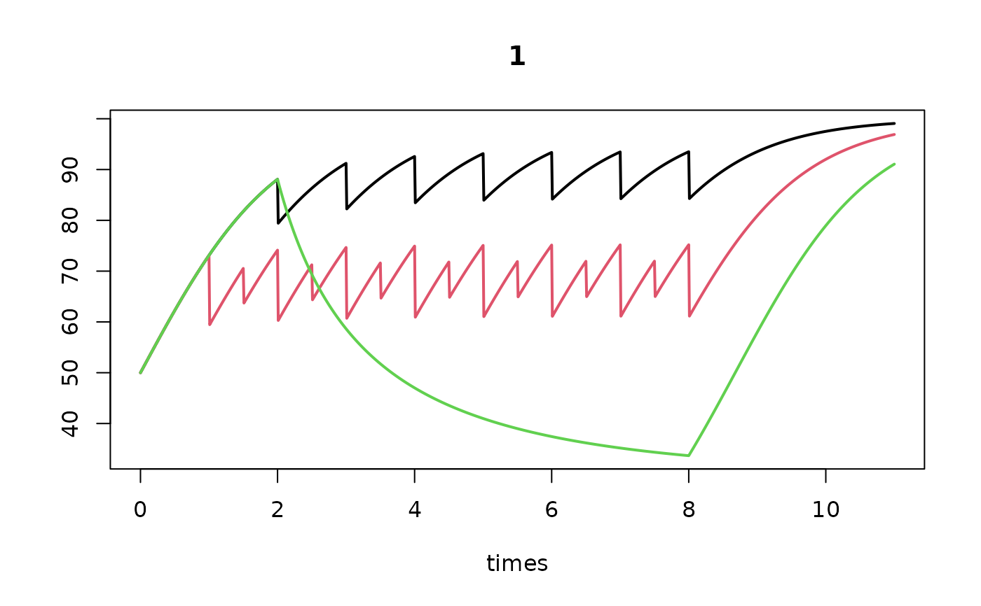
## ====================================================
## Simple runs
## ====================================================
times <- seq(0, 11, by = 0.01)
T1 <- density_perturb (K = 100, D0 = 50,
tstart_perturb = 2,
tend_perturb = 8,
times = times)
T2 <- density_metier (K = 100, D0 = 50, sar = data.frame(1, 2),
tstart_perturb = 1,
tend_perturb = 8,
times = times)
T3 <- density_logistic (K = 100, r = 1, m = 0.7, D0 = 50,
tstart_perturb = 2,
tend_perturb = 8,
times = times)
plot(T1, T2, T3, lty = 1, lwd = 2)
 ## ====================================================
## Compare density_perturb with dynamic run_perturb
## ====================================================
times <- c(0, 0.5, 1.5, 2.5, 8.5)
T1 <- density_perturb (K = 100,
tstart_perturb = 0,
times = times)
T1
#> times 1
#> 1 0.0 90.00000
#> 2 0.5 93.68627
#> 3 1.5 91.32927
#> 4 2.5 90.39963
#> 5 8.5 89.77085
# dynamic run
rP <- run_perturb(parms = list(K = 100, r = 1, d = 0.1),
sar = 1,
times = seq(0, 11, by = 0.01))
# compare
plot(rP, ylim = c(80, 100), las = 1,
main = "comparison density_perturb and run_perturb")
points(T1,
pch = 16, cex = 2)
legend("topright",
legend = c("run_perturb",
"density_perturb"),
lty = c(1, NA), pch = c(NA, 16))
## ====================================================
## Compare density_perturb with dynamic run_perturb
## ====================================================
times <- c(0, 0.5, 1.5, 2.5, 8.5)
T1 <- density_perturb (K = 100,
tstart_perturb = 0,
times = times)
T1
#> times 1
#> 1 0.0 90.00000
#> 2 0.5 93.68627
#> 3 1.5 91.32927
#> 4 2.5 90.39963
#> 5 8.5 89.77085
# dynamic run
rP <- run_perturb(parms = list(K = 100, r = 1, d = 0.1),
sar = 1,
times = seq(0, 11, by = 0.01))
# compare
plot(rP, ylim = c(80, 100), las = 1,
main = "comparison density_perturb and run_perturb")
points(T1,
pch = 16, cex = 2)
legend("topright",
legend = c("run_perturb",
"density_perturb"),
lty = c(1, NA), pch = c(NA, 16))
 ## ====================================================
## Compare density_logistic with dynamic run_logistic
## ====================================================
times <- c(0, 0.5, 1.5, 2.5, 8.5)
T2 <- density_logistic(K = 100,
times = times)
T2
#> times 1
#> 1 0.0 100.00000
#> 2 0.5 96.12949
#> 3 1.5 92.39526
#> 4 2.5 90.95870
#> 5 8.5 90.00428
# dynamic run
rL <- run_logistic(parms = list(K = 100, r = 1, m = 0.1),
times = seq(0, 11, by = 0.01))
# compare
plot(rL, ylim = c(80, 100), las = 1,
main = "comparison density_logistic and run_logistic")
points(T2,
pch = 18, cex = 2)
legend("topright",
legend = c("run_logistic",
"density_logistic"),
lty = c(1, NA), pch = c(NA, 18))
## ====================================================
## Compare density_logistic with dynamic run_logistic
## ====================================================
times <- c(0, 0.5, 1.5, 2.5, 8.5)
T2 <- density_logistic(K = 100,
times = times)
T2
#> times 1
#> 1 0.0 100.00000
#> 2 0.5 96.12949
#> 3 1.5 92.39526
#> 4 2.5 90.95870
#> 5 8.5 90.00428
# dynamic run
rL <- run_logistic(parms = list(K = 100, r = 1, m = 0.1),
times = seq(0, 11, by = 0.01))
# compare
plot(rL, ylim = c(80, 100), las = 1,
main = "comparison density_logistic and run_logistic")
points(T2,
pch = 18, cex = 2)
legend("topright",
legend = c("run_logistic",
"density_logistic"),
lty = c(1, NA), pch = c(NA, 18))
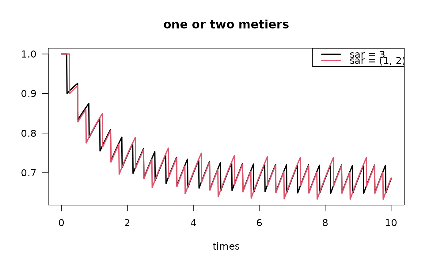
 ## ====================================================
## Several metiers, one taxon
## ====================================================
times <- seq(0, 10, length.out = 1000)
sar = data.frame(1, 2) # 2 metiers
M1 <- density_metier (times = times,
K = 1, r = 1,
d = data.frame(0.1, 0.1),
sar = sar,
as.deSolve = TRUE)
# Compare with one metier run,
P1 <- density_perturb(times = times,
K = 1, r = 1, d = 0.1,
sar = sum(sar), # sum of sar
as.deSolve = TRUE)
plot(P1, M1, lty = 1, main = "one or two metiers",
las = 1, lwd = 2)
legend("topright", col = 1:2, lty = 1, lwd = 2,
legend = c("sar = 3", "sar = (1, 2)"))
## ====================================================
## Several metiers, one taxon
## ====================================================
times <- seq(0, 10, length.out = 1000)
sar = data.frame(1, 2) # 2 metiers
M1 <- density_metier (times = times,
K = 1, r = 1,
d = data.frame(0.1, 0.1),
sar = sar,
as.deSolve = TRUE)
# Compare with one metier run,
P1 <- density_perturb(times = times,
K = 1, r = 1, d = 0.1,
sar = sum(sar), # sum of sar
as.deSolve = TRUE)
plot(P1, M1, lty = 1, main = "one or two metiers",
las = 1, lwd = 2)
legend("topright", col = 1:2, lty = 1, lwd = 2,
legend = c("sar = 3", "sar = (1, 2)"))
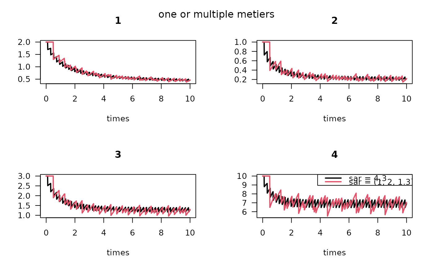
 ## ====================================================
## Several metiers, multiple taxa
## ====================================================
times <- seq(0, 10, length.out = 1000)
# 4 taxa, 3 metiers
d <- data.frame(sar1 = c(0.1, 0.2, 0.15, 0.2),
sar2 = c(0.2, 0.3, 0.25, 0.1),
sar3 = c(0.1, 0.3, 0.01, 0.1))
K <- c(2, 1, 3, 10)
r <- c(1, 2, 1.5, 2)
sar <- data.frame(1, 2.5, 1.3)
M1 <- density_metier (times = times,
K = K, r = r,
d = d,
sar = sar,
as.deSolve = TRUE)
# compare with the single metier model
# average depletion
d1 <- (d[,1]*sar[[1]] + d[,2]*sar[[2]] + d[,3]*sar[[3]])/sum(sar)
P1 <- density_perturb(times = times,
K = K, r = r,
d = d1,
sar = sum(sar),
as.deSolve = TRUE)
plot(P1, M1, lty = 1,
las = 1, lwd = 2)
legend("topright", col = 1:2, lty = 1, lwd = 2,
legend = c("sar = 4.3", "sar = (1, 2, 1.3)"))
mtext(side = 3, line = -2, "one or multiple metiers", outer = TRUE)
## ====================================================
## Several metiers, multiple taxa
## ====================================================
times <- seq(0, 10, length.out = 1000)
# 4 taxa, 3 metiers
d <- data.frame(sar1 = c(0.1, 0.2, 0.15, 0.2),
sar2 = c(0.2, 0.3, 0.25, 0.1),
sar3 = c(0.1, 0.3, 0.01, 0.1))
K <- c(2, 1, 3, 10)
r <- c(1, 2, 1.5, 2)
sar <- data.frame(1, 2.5, 1.3)
M1 <- density_metier (times = times,
K = K, r = r,
d = d,
sar = sar,
as.deSolve = TRUE)
# compare with the single metier model
# average depletion
d1 <- (d[,1]*sar[[1]] + d[,2]*sar[[2]] + d[,3]*sar[[3]])/sum(sar)
P1 <- density_perturb(times = times,
K = K, r = r,
d = d1,
sar = sum(sar),
as.deSolve = TRUE)
plot(P1, M1, lty = 1,
las = 1, lwd = 2)
legend("topright", col = 1:2, lty = 1, lwd = 2,
legend = c("sar = 4.3", "sar = (1, 2, 1.3)"))
mtext(side = 3, line = -2, "one or multiple metiers", outer = TRUE)