Sensitivity of an area or taxon to fishing parameters
sensitivity.Rdsensitivity_taxon estimates for one taxon the density decrease for combinations of sar and gpd;
also estimates critical (sar x gpd) values for the taxon.
sensitivity_area estimates for one set of sar and gpd values the density decrease for combinations of r (rate of natural increase) and d (depletion);
also estimates critical (r x d) combinations for the area.
Arguments
- sar, sar.seq
fishing intensity, estimated as Swept Area Ratio, units e.g. [m2/m2/year]. One number defining the area (
sensitivity_area), or a vector (sensitivity_taxon) for which sensitivity needs to be estimated.- gpd, gpd.seq
gear penetration depth, units e.g. [cm]. One number defining the area (
sensitivity_area), or a vector (sensitivity_taxon) for which sensitivity needs to be estimated.- r, r.seq
the rate of increase of each taxon, units e.g. [/year]. One number defining the taxon (
sensitivity_taxon), or a vector (sensitivity_area) for which sensitivity needs to be estimated.- d.seq
depletion fraction due to fishing, a vector (
sensitivity_area) for which sensitivity needs to be estimated.- fDepth
fractional occurrence of species in sediment layers, dimensionless. A vector of the same length as
uDepth. The sum offDepthshould equal 1. Will be used to estimate the depletion fractiond.- uDepth
depth of the upper position of the sediment layers, units e.g. [cm]. A vector with length equal to the number of columns of
fDepth.- ...
arguments passed to the
par_dfunction
Value
function sensitivity_taxon returns a list with:
sar, the sequence of swept area ratios corresponding toDK, [/year]gpd, the sequence of gear penetration depths corresponding toDK, [cm]DK, the density/carrying capacity ratio, a matrix, corresponding tosar(rows) andgpd(column), [-]critical_sar, the critical value ofsarfor eachgpd, above which the taxon is extinct, [/yr]critical_gpd, the critical value ofgpdfor eachsar, above which the taxon is extinct, [cm]r, the intrinsic rate of natural increase of the taxon, [/yr]Depth_mean, the mean living depth of the taxon (sum(fDepth*uDepth)), [cm]d_mean, the mean depletion fraction (for each gpd), [-]
function sensitivity_area returns a list with:
r, the sequence of intrinsic rate of natural increase, corresponding toDK, [/year]d, the sequence of d, depletion fractions, corresponding toDK, [cm]DK, the density/carrying capacity ratio, a matrix, corresponding tor(rows) andd(column), [-]critical_r, the critical value ofrfor eachd, below which the taxon is extinct, [/yr]critical_d, the critical value ofdfor eachr, above which the taxon is extinct, [-]sar, the swept area ratio of the area, [/yr]gpd, the gear penetration depth of the area, [cm]
See also
run_perturb for how to run a disturbance model.
Traits_nioz, for trait databases in package Btrait.
MWTL for data sets on which fishing can be imposed.
map_key for simple plotting functions.
Examples
## -----------------------------------------------------------------------
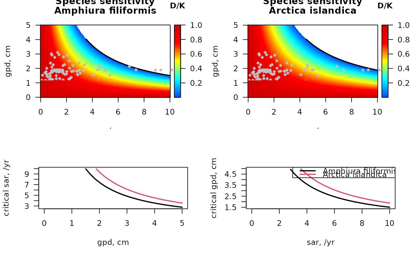
## sensitivity for two species in the Dutch part of the Northsea
## -----------------------------------------------------------------------
par(mfrow = c(2,2), las = 1)
# parameters for A. filiformis and for Arctica islandica
subset(MWTL$fishing,
subset = (taxon == "Amphiura filiformis"))
#> taxon p0 p0_5cm p5_15cm p15_30cm p30cm Age.at.maturity r
#> 25 Amphiura filiformis 0 0.75 0.25 0 0 4 0.64
S_af <- sensitivity_taxon(r = 0.64,
fDepth = c(0.75, 0.25),
uDepth = c(0, 5))
subset(MWTL$fishing,
subset = (taxon == "Arctica islandica"))
#> taxon p0 p0_5cm p5_15cm p15_30cm p30cm Age.at.maturity r
#> 38 Arctica islandica 0 0.6 0.4 0 0 4 0.64
S_ai <- sensitivity_taxon(r = 0.64,
fDepth = c(0.6, 0.4),
uDepth = c(0, 5))
# image, black = extinct
image2D(x = S_af$sar, y = S_af$gpd, z = S_af$DK,
xlab = "sar, /yr", ylab = "gpd, cm",
main = c("Species sensitivity",
"Amphiura filiformis"),
col = jet2.col(100), clab = "D/K")
lines(S_af$sar, S_af$critical_gpd, lwd = 2)
# add the stations in the MWTL data (from Btrait)
points(MWTL$abiotics$sar, MWTL$abiotics$gpd,
pch = 18, col = "grey")
# image, blue = extinct
image2D(x = S_ai$sar, y = S_ai$gpd, z = S_ai$DK,
xlab = "sar, /yr", ylab = "gpd, cm",
main = c("Species sensitivity",
"Arctica islandica"),
col = jet2.col(100), clab = "D/K")
lines(S_ai$sar, S_ai$critical_gpd, lwd = 2)
# add the stations in the MWTL data (from Btrait)
points(MWTL$abiotics$sar, MWTL$abiotics$gpd,
pch = 18, col = "grey")
matplot(S_af$gpd, cbind(S_af$critical_sar, S_ai$critical_sar),
xlab = "gpd, cm", ylab = "critical sar, /yr",
type = "l", lty = 1, lwd = 2)
matplot(S_af$sar, cbind(S_af$critical_gpd, S_ai$critical_gpd),
xlab = "sar, /yr", ylab = "critical gpd, cm",
type = "l", lty = 1, lwd = 2)
legend("topright", col = 1:2, lty = 1, lwd = 2,
legend = c("Amphiura filiformis", "Arctica islandica"))
 ## -----------------------------------------------------------------------
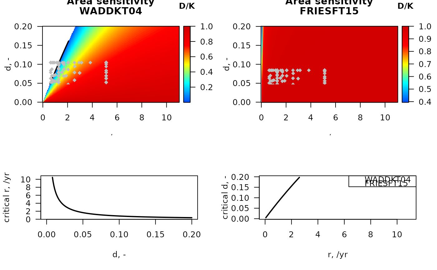
## sensitivity for two stations in the Dutch part of the Northsea
## -----------------------------------------------------------------------
par(mfrow = c(2, 2), las = 1)
# parameters for stations WADDKT04, FRIESFT15
subset(MWTL$abiotics,
subset = (station== "WADDKT04"),
select = c(station, sar, gpd))
#> station sar gpd
#> 97 WADDKT04 11.81742 1.898136
S_W <- sensitivity_area(sar = 11.817,
gpd = 1.90,
r.seq = seq(0, 11, length.out = 200),
d.seq = seq(0, 0.2, length.out = 200))
subset(MWTL$abiotics,
subset = (station == "FRIESFT15"),
select = c(station, sar, gpd))
#> station sar gpd
#> 48 FRIESFT15 0.1466945 1.52917
S_F <- sensitivity_area(sar = 0.15,
gpd = 1.53,
r.seq = seq(0, 11, length.out = 200),
d.seq = seq(0, 0.2, length.out = 200))
# The species in the MWTL data (from Btrait)
Fish <- MWTL$fishing
# depletion for all MWTL species in station WADDKT04
Fish$dW <- par_d(
gpd = 1.90,
fDepth = Fish[, c("p0", "p0_5cm", "p5_15cm", "p15_30cm", "p30cm")],
uDepth = c( 0, 0, 5, 15, 30))
# depletion for all MWTL species in station FRIESFT15
Fish$dF <- par_d(
gpd = 1.53,
fDepth = Fish[, c("p0", "p0_5cm", "p5_15cm", "p15_30cm", "p30cm")],
uDepth = c( 0, 0, 5, 15, 30))
# image of station sensitivity, white = extinct (D/K = NA)
image2D(x = S_W$r, y = S_W$d, z=S_W$DK,
xlab = "r, /yr", ylab = "d, -",
main = c("Area sensitivity",
"WADDKT04"),
col = jet2.col(100), clab = "D/K")
lines(S_W$r, S_W$critical_d, lwd = 2)
points(Fish$r, Fish$dW,
pch = 18, col = "grey")
# image, white = extinct (D/K = NA)
image2D(x = S_F$r, y = S_F$d, z=S_F$DK,
xlab = "r, /yr", ylab = "d, -",
main = c("Area sensitivity",
"FRIESFT15"),
col = jet2.col(100), clab = "D/K")
lines(S_F$r, S_F$critical_d, lwd = 2)
points(Fish$r, Fish$dF,
pch = 18, col = "grey")
matplot(S_W$d, cbind(S_W$critical_r, S_F$critical_r),
xlab = "d, -", ylab = "critical r, /yr",
type = "l", lty = 1, lwd = 2)
matplot(S_W$r, cbind(S_W$critical_d, S_F$critical_d),
xlab = "r, /yr", ylab = "critical d, -",
type = "l", lty = 1, lwd = 2)
legend("topright", col = 1:2,
legend = c("WADDKT04", "FRIESFT15"))
## -----------------------------------------------------------------------
## sensitivity for two stations in the Dutch part of the Northsea
## -----------------------------------------------------------------------
par(mfrow = c(2, 2), las = 1)
# parameters for stations WADDKT04, FRIESFT15
subset(MWTL$abiotics,
subset = (station== "WADDKT04"),
select = c(station, sar, gpd))
#> station sar gpd
#> 97 WADDKT04 11.81742 1.898136
S_W <- sensitivity_area(sar = 11.817,
gpd = 1.90,
r.seq = seq(0, 11, length.out = 200),
d.seq = seq(0, 0.2, length.out = 200))
subset(MWTL$abiotics,
subset = (station == "FRIESFT15"),
select = c(station, sar, gpd))
#> station sar gpd
#> 48 FRIESFT15 0.1466945 1.52917
S_F <- sensitivity_area(sar = 0.15,
gpd = 1.53,
r.seq = seq(0, 11, length.out = 200),
d.seq = seq(0, 0.2, length.out = 200))
# The species in the MWTL data (from Btrait)
Fish <- MWTL$fishing
# depletion for all MWTL species in station WADDKT04
Fish$dW <- par_d(
gpd = 1.90,
fDepth = Fish[, c("p0", "p0_5cm", "p5_15cm", "p15_30cm", "p30cm")],
uDepth = c( 0, 0, 5, 15, 30))
# depletion for all MWTL species in station FRIESFT15
Fish$dF <- par_d(
gpd = 1.53,
fDepth = Fish[, c("p0", "p0_5cm", "p5_15cm", "p15_30cm", "p30cm")],
uDepth = c( 0, 0, 5, 15, 30))
# image of station sensitivity, white = extinct (D/K = NA)
image2D(x = S_W$r, y = S_W$d, z=S_W$DK,
xlab = "r, /yr", ylab = "d, -",
main = c("Area sensitivity",
"WADDKT04"),
col = jet2.col(100), clab = "D/K")
lines(S_W$r, S_W$critical_d, lwd = 2)
points(Fish$r, Fish$dW,
pch = 18, col = "grey")
# image, white = extinct (D/K = NA)
image2D(x = S_F$r, y = S_F$d, z=S_F$DK,
xlab = "r, /yr", ylab = "d, -",
main = c("Area sensitivity",
"FRIESFT15"),
col = jet2.col(100), clab = "D/K")
lines(S_F$r, S_F$critical_d, lwd = 2)
points(Fish$r, Fish$dF,
pch = 18, col = "grey")
matplot(S_W$d, cbind(S_W$critical_r, S_F$critical_r),
xlab = "d, -", ylab = "critical r, /yr",
type = "l", lty = 1, lwd = 2)
matplot(S_W$r, cbind(S_W$critical_d, S_F$critical_d),
xlab = "r, /yr", ylab = "critical d, -",
type = "l", lty = 1, lwd = 2)
legend("topright", col = 1:2,
legend = c("WADDKT04", "FRIESFT15"))
 ## -----------------------
## sensitivity_taxon
## -----------------------
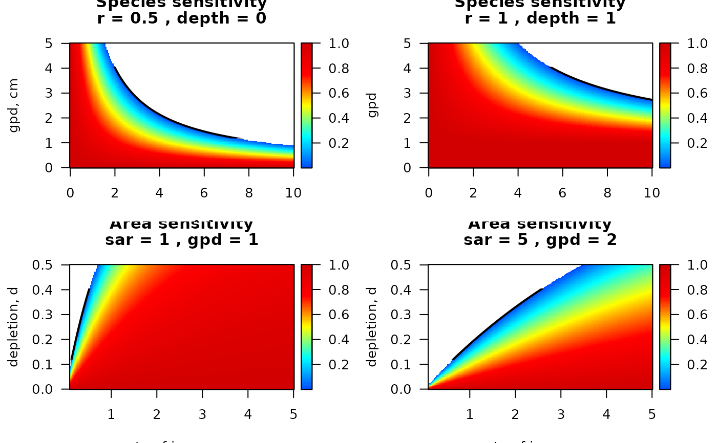
par(las = 1, mfrow = c(2,2))
S_sp1 <- sensitivity_taxon(r = 0.5)
image2D(x = S_sp1$sar, y = S_sp1$gpd, z=S_sp1$DK,
xlab = "sar, yr^-1", ylab = "gpd, cm",
main = c("Species sensitivity",
paste0("r = ", S_sp1$r,
" , depth = ", S_sp1$Depth_mean)),
col = jet2.col(100))
lines(S_sp1$sar, S_sp1$critical_gpd, lwd = 2)
S_sp2 <- sensitivity_taxon(r = 1, uDepth = 1)
image2D(x = S_sp2$sar, y = S_sp2$gpd, z=S_sp2$DK,
col = jet2.col(100),
xlab = "sar", ylab = "gpd",
main = c("Species sensitivity",
paste0("r = ", S_sp2$r,
" , depth = ", S_sp2$Depth_mean)))
lines(S_sp2$sar, S_sp2$critical_gpd, lwd = 2)
## -----------------------
## sensitivity_area
## -----------------------
AA <- sensitivity_area(sar = 1, gpd = 1)
image2D(x = AA$r, y = AA$d, z=AA$DK, col = jet2.col(100),
xlab = "rate of increase, r", ylab = "depletion, d",
main = c("Area sensitivity",
paste0("sar = ", AA$sar, " , gpd = ", AA$gpd)))
lines(AA$r, AA$critical_d, lwd = 2)
A2 <- sensitivity_area(sar = 5, gpd = 2)
image2D(x = A2$r, y = A2$d, z=A2$DK,
col = jet2.col(100),
xlab = "rate of increase, r", ylab = "depletion, d",
main = c("Area sensitivity",
paste0("sar = ", A2$sar, " , gpd = ", A2$gpd)))
lines(A2$r, A2$critical_d, lwd = 2)
## -----------------------
## sensitivity_taxon
## -----------------------
par(las = 1, mfrow = c(2,2))
S_sp1 <- sensitivity_taxon(r = 0.5)
image2D(x = S_sp1$sar, y = S_sp1$gpd, z=S_sp1$DK,
xlab = "sar, yr^-1", ylab = "gpd, cm",
main = c("Species sensitivity",
paste0("r = ", S_sp1$r,
" , depth = ", S_sp1$Depth_mean)),
col = jet2.col(100))
lines(S_sp1$sar, S_sp1$critical_gpd, lwd = 2)
S_sp2 <- sensitivity_taxon(r = 1, uDepth = 1)
image2D(x = S_sp2$sar, y = S_sp2$gpd, z=S_sp2$DK,
col = jet2.col(100),
xlab = "sar", ylab = "gpd",
main = c("Species sensitivity",
paste0("r = ", S_sp2$r,
" , depth = ", S_sp2$Depth_mean)))
lines(S_sp2$sar, S_sp2$critical_gpd, lwd = 2)
## -----------------------
## sensitivity_area
## -----------------------
AA <- sensitivity_area(sar = 1, gpd = 1)
image2D(x = AA$r, y = AA$d, z=AA$DK, col = jet2.col(100),
xlab = "rate of increase, r", ylab = "depletion, d",
main = c("Area sensitivity",
paste0("sar = ", AA$sar, " , gpd = ", AA$gpd)))
lines(AA$r, AA$critical_d, lwd = 2)
A2 <- sensitivity_area(sar = 5, gpd = 2)
image2D(x = A2$r, y = A2$d, z=A2$DK,
col = jet2.col(100),
xlab = "rate of increase, r", ylab = "depletion, d",
main = c("Area sensitivity",
paste0("sar = ", A2$sar, " , gpd = ", A2$gpd)))
lines(A2$r, A2$critical_d, lwd = 2)